Review purpose:

Better understand the basic model idea and principle implementation of the annealing algorithm, and further optimize the previous implementation code

On the basis of the original annealing algorithm, the possibility of "dead ash reburning" is introduced, which reduces the fluctuation degree of the algorithm results and improves the optimization degree of the solution.

Part I:

Calculate the distance between all points (energy meter)

function [ fare ] = distance( coord )
% Find the distance between each city according to its distance coordinate
% fare For the distance between cities, coord Coordinates for each city
[ v , m ] = size( coord ) ; % m Number of cities
fare = zeros( m ) ;
for i = 1 : m % Outer row
for j = i : m % Inner layer is column
fare( i , j ) = ( sum( ( coord( : , i ) - coord( : , j ) ) .^ 2 ) ) ^ 0.5 ;
fare( j , i ) = fare( i , j ) ; % Distance matrix symmetry
end
end

Part II:

Calculate the energy value (cost value) generated by the path planning, fare: energy meter

function [ objval ] = pathfare( fare , path )
% Calculation path path The price of objval
% path For 1 to n , which represents the visiting order of the city;
% fare Is a cost matrix, and is a square matrix.
[ m , n ] = size( path ) ;
objval = zeros( 1 , m ) ;
for i = 1 : m
for j = 2 : n
objval( i ) = objval( i ) + fare( path( i , j - 1 ) , path( i , j ) ) ;
end
objval( i ) = objval( i ) + fare( path( i , n ) , path( i , 1 ) ) ;
end

Part three:

It is to generate a new searchable path through the position exchange of several "position point pairs".

function [ newpath , position ] = swap( oldpath , number )
% Yes oldpath Exchange operation
% number Is the number of new paths generated
% position Corresponding newpath Swap location
m = length( oldpath ) ; % Number of cities
newpath = zeros( number , m ) ;
position = sort( randi( m , number , 2 ) , 2 ); % The location of randomly generated exchanges,Sort each pair of swap points
for i = 1 : number
newpath( i , : ) = oldpath ;
% City selected in swap path
newpath( i , position( i , 1 ) ) = oldpath( position( i , 2 ) ) ;
newpath( i , position( i , 2 ) ) = oldpath( position( i , 1 ) ) ;
end

Part four:

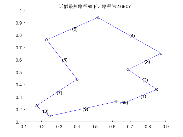
First, draw the position circle points through coordinates, and then draw the line according to the optimal path.

function [ ] = myplot( path , coord , pathfar )
% Figure making path
% path For the path to be mapped, coord Coordinates for each city
% pathfar As path path Corresponding expenses
len = length( path ) ;
clf ;
hold on ;
title( [ 'The approximate shortest path is' , num2str( pathfar ) ] ) ;
plot( coord( 1 , : ) , coord( 2 , : ) , 'ok');
pause( 0.4 ) ;
for ii = 2 : len
plot( coord( 1 , path( [ ii - 1 , ii ] ) ) , coord( 2 , path( [ ii - 1 , ii ] ) ) , '-b');
x = sum( coord( 1 , path( [ ii - 1 , ii ] ) ) ) / 2 ;
y = sum( coord( 2 , path( [ ii - 1 , ii ] ) ) ) / 2 ;
text( x , y , [ '(' , num2str( ii - 1 ) , ')' ] ) ;
pause( 0.4 ) ;
end
plot( coord( 1 , path( [ 1 , len ] ) ) , coord( 2 , path( [ 1 , len ] ) ) , '-b' ) ;
x = sum( coord( 1 , path( [ 1 , len ] ) ) ) / 2 ;
y = sum( coord( 2 , path( [ 1 , len ] ) ) ) / 2 ;
text( x , y , [ '(' , num2str( len ) , ')' ] ) ;
pause( 0.4 ) ;
hold off ;

Part V:

Two level iteration: the inner layer generates new optimal state; the outer layer records the historical optimal state of all the inner layers

The inner layer shows dynamic thermal change, and the outer layer shows annealing phenomenon in general.

The stability criterion of Metropolis sampling determines whether it is possible to reach the ideal value. Random Rand < 0.1 is to avoid the phenomenon of "resurgence", so as to achieve the effect that the sampling criterion cannot achieve.

clear;
% Program parameter setting
Coord = ... % City coordinates Coordinates
[ 0.6683 0.6195 0.4    0.2439 0.1707 0.2293 0.5171 0.8732 0.6878 0.8488 ; ...
  0.2536 0.2634 0.4439 0.1463 0.2293 0.761  0.9414 0.6536 0.5219 0.3609 ] ;
t0 = 1 ; % Initial temperature t0
iLk = 20 ; % Maximum number of iterations of inner cycle iLk
oLk = 1000 ; % Maximum iterations of external cycle oLk
lam = 0.95 ; % λ lambda
istd = 0.00001 ; % If the variance of the value of the inner loop function is less than istd Then stop
ostd = 0.00001 ; % If the variance of the value of the outer loop function is less than ostd Then stop
ilen = 5 ; % Number of objective function values saved in inner loop
olen = 5 ; % Number of objective function values saved in the outer loop
% Program subject
m = length( Coord ) ; % Number of cities m
fare = distance( Coord ) ; % Path cost fare
path = 1 : m ; % Initial path path
pathfar = pathfare( fare , path ) ; % Path cost path fare
ores = zeros( 1 , olen ) ; % Objective function value saved by outer loop
e0 = pathfar ; % Initial value of energy e0
t = t0 ; % Temperature t
for out = 1 : oLk % External circulation simulated annealing process
    ires = zeros( 1 , ilen ) ; % Objective function value stored in inner loop
    for in = 1 : iLk % Internal circulation simulation of heat balance process
        [ newpath , v ] = swap( path , 1 ) ; % Create a new state
        e1 = pathfare( fare , newpath ) ; % New state energy
        % Metropolis Sampling stability criteria
        r = min( 1 , exp( - ( e1 - e0 ) / t ) ) ;
        if rand < r
            path = newpath ; % Update best
            e0 = e1 ;
        end
        ires = [ ires( 2 : end ) e0 ] ; % Save new state energy
        % Internal circulation termination criterion: continuous ilen State energy fluctuation less than istd
        if std( ires , 1 ) < istd %Divide by call n Standard deviation function of
            if rand < 0.1 %Increase the possibility of a mutation
                break ;
            end
        end
    end
    ores = [ ores( 2 : end ) e0 ] ; % Save new state energy
    % External circulation termination criterion: continuous olen State energy fluctuation less than ostd
    if std( ores , 1 ) < ostd
        if rand < 0.1 %Increase the possibility of a mutation
            break ;
        end
    end
    t = lam * t ;
end
pathfar = e0 ;
% Enter results
fprintf( 'The approximate optimal path is:\n ' )
%disp( char( [ path , path(1) ] + 64 ) ) ;
disp(path)
fprintf( 'Approximate optimal path path\tpathfare=' ) ;
disp( pathfar ) ;
myplot( path , Coord , pathfar ) ;

The final result is very stable (the fluctuation value is basically between 2.6907 and 2.7):