ResNet, an article published by he Kaiming on CVPR in 2015, uses the concept of residual connection. As soon as the paper was published, it directly detonated the whole cv world. And ResNet won the first place on ImageNet in 2016. ResNet has been used in cutting-edge technologies in various fields of AI.
I would be satisfied if I cited one tenth of ResNet in my future papers (laughter)
Introduction to ResNet
ResNet solves the problem of deep network degradation. Generally speaking, the deeper the network, the more complex the results can be fitted by the model. However, in the actual training, once the model is deepened, the effect is not necessarily good, and it is likely to have some disadvantages, such as poor fitting effect, gradient disappearance and so on. For example, the test accuracy of 20 layer CNN and 56 layer CNN on CIFAR-10 shown in the paper. It can be seen from the figure that the accuracy of 56 layer CNN is worse than that of 20 layer CNN.
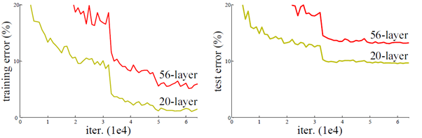
In the training process, when the network returns, the gradient of each layer of the network is obtained and multiplied. The more the network is trained to the later stage or deeper, its gradient is very small, so the total gradient obtained after multiplication is very few or even close to 0. In order to solve this problem, Dr. he put forward the concept of residual learning in his paper.
Residual learning
When we need to add several layers of networks on the basis of a network, the conventional practice is to add the network directly behind, and the output of the original network is added with the input of the network. But now we don't do this. According to residual learning, when the input of the new network is x, the learned feature is recorded as H (x) , Now we hope that the new network can learn the residual value F(x)=H(x)-x , In fact, the original learning characteristics are F(x)+x . In other words, for the final output, we still need to add x to f (x).
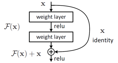
Adding a new network to the original network is easy to make the network degradation gradient very small. When the output is changed to the sum of the residual value and the network value, there will be no value that produces a small gradient when calculating the gradient. Because there is an x in the derivation formula, it is well known that when we derive a variable, the derivative of x is 1. It can also be said that the gradient obtained by deriving the network of this layer is a small gradient plus a 1. This increases the value of the gradient and makes up for the disadvantage that the gradient will disappear. Of course, the residual gradient will not be all 1, and even if it is relatively small, the existence of 1 will not cause the gradient to disappear. So residual learning will be easier.
network structure
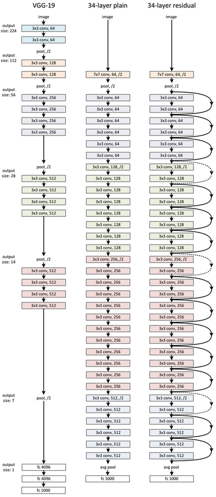
The network similar to VGG is adopted and improved, and the residual unit is added through the short-circuit mechanism. The basic unit structure is still the routine of convolution, BN and activation function. However, the residual connection is added to the output position of each unit. The unit output plus the unit input is finally used as the final output through an activation function.
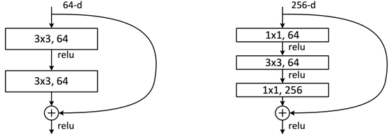
For different layers of ResNet, the structure of residual unit is also different
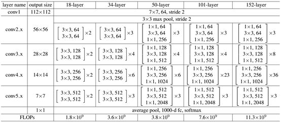
When it is less than 50 layers, there are only two convolutions in the general residual unit, and one convolution is the size of 3 * 3 convolution kernel, and then the filling is 1, which does not change the size of the feature map, while the other convolution reduces the size by half. This operation doubles the number of channels of the feature map in order not to lose too much information, and also reduces the complexity of the network. When it is greater than 50 layers, first use a 1 * 1 convolution layer to map the number of channels of the feature map back to the number of channels I need, and then use the same 3 * 3 convolution layer to change the size as above. Finally, it passes through a convolution layer that multiplies the number of channels by four times. As can be seen from the figure, ResNet adds a short circuit mechanism between each two layers compared with ordinary networks, which forms residual learning. The dotted line indicates that the number of feature maps has changed.
Python implements ResNet
import torch
import time
from torch import nn

# The initial convolution layer processes the input image into a feature map
class Conv1(nn.Module):
    def __init__(self,inp_channels,out_channels,stride = 2):
        super(Conv1,self).__init__()
        self.net = nn.Sequential(
            nn.Conv2d(inp_channels,out_channels,kernel_size=7,stride=stride,padding=3,bias=False),# The result of convolution is (i - k + 2*p)/s + 1, and the image size is reduced by half
            nn.BatchNorm2d(out_channels),
            nn.ReLU(inplace=True),
            nn.MaxPool2d(kernel_size=3,stride=2,padding=1)# According to the convolution formula, the feature map size becomes half of the original size
        )

    def forward(self,x):
        y = self.net(x)
        return y

class Simple_Res_Block(nn.Module):
    def __init__(self,inp_channels,out_channels,stride=1,downsample = False,expansion_=False):
        super(Simple_Res_Block,self).__init__()
        self.downsample = downsample
        if expansion_:
            self.expansion = 4# Expand dimension to expansion times
        else:
            self.expansion = 1

        self.block = nn.Sequential(
            nn.Conv2d(inp_channels,out_channels,kernel_size=3,stride=stride,padding=1),
            nn.BatchNorm2d(out_channels),
            nn.ReLU(inplace=True),
            nn.Conv2d(out_channels,out_channels*self.expansion,kernel_size=3,padding=1),
            nn.BatchNorm2d(out_channels*self.expansion)
        )
        if self.downsample:
            self.down = nn.Sequential(
                nn.Conv2d(inp_channels,out_channels*self.expansion,kernel_size=1,stride=stride,bias=False),
                nn.BatchNorm2d(out_channels*self.expansion)
            )
        self.relu = nn.ReLU(inplace=True)

    def forward(self,input):
        residual = input
        x = self.block(input)
        if self.downsample:
            residual = self.down(residual)# Make the dimensions of x and h the same

        out = residual + x
        out = self.relu(out)
        return out

class Residual_Block(nn.Module):
    def __init__(self,inp_channels,out_channels,stride=1,downsample = False,expansion_=False):
        super(Residual_Block,self).__init__()
        self.downsample = downsample# Judge whether to down sample x so that the number of dimension channels of x and the output value of the module is the same
        if expansion_:
            self.expansion = 4# Expand dimension to expansion times
        else:
            self.expansion = 1

        # modular
        self.conv1 = nn.Conv2d(inp_channels,out_channels,kernel_size=1,stride=1,bias=False)# It does not change the size of the feature map and plays a mapping role
        self.drop = nn.Dropout(0.5)
        self.BN1 = nn.BatchNorm2d(out_channels)
        self.conv2 = nn.Conv2d(out_channels,out_channels,kernel_size=3,stride=stride,padding=1,bias=False)# At this time, the size of convolution kernel and filling size will not affect the size of feature graph, which is determined by step size
        self.BN2 = nn.BatchNorm2d(out_channels)
        self.conv3 = nn.Conv2d(out_channels,out_channels*self.expansion,kernel_size=1,stride=1,bias=False)# Change the number of channels
        self.BN3 = nn.BatchNorm2d(out_channels*self.expansion)
        self.relu = nn.ReLU(inplace=True)

        if self.downsample:
            self.down = nn.Sequential(
                nn.Conv2d(inp_channels,out_channels*self.expansion,kernel_size=1,stride=stride,bias=False),
                nn.BatchNorm2d(out_channels*self.expansion)
            )

    def forward(self,input):
        residual = input
        x = self.relu(self.BN1(self.conv1(input)))
        x = self.relu(self.BN2(self.conv2(x)))
        h = self.BN3(self.conv3(x))

        if self.downsample:
            residual = self.down(residual)# Make the dimensions of x and h the same
        out = h + residual# Residual part
        out = self.relu(out)
        return out

class Resnet(nn.Module):
    def __init__(self,net_block,block,num_class = 1000,expansion_=False):
        super(Resnet,self).__init__()
        self.expansion_ = expansion_
        if expansion_:
            self.expansion = 4# Expand dimension to expansion times
        else:
            self.expansion = 1

        # Convolution of the input initial image
        # (3*64*64) --> (64*56*56)
        self.conv = Conv1(3,64)

        # Building blocks
        # (64*56*56) --> (256*56*56)
        self.block1 = self.make_layer(net_block,block[0],64,64,expansion_=self.expansion_,stride=1)# Stripe is 1, and the size is not changed
        # (256*56*56) --> (512*28*28)
        self.block2 = self.make_layer(net_block,block[1],64*self.expansion,128,expansion_=self.expansion_,stride=2)
        # (512*28*28) --> (1024*14*14)
        self.block3 = self.make_layer(net_block,block[2],128*self.expansion,256,expansion_=self.expansion_,stride=2)
        # (1024*14*14) --> (2048*7*7)
        self.block4 = self.make_layer(net_block,block[3],256*self.expansion,512,expansion_=self.expansion_,stride=2)

        self.avgPool = nn.AvgPool2d(7,stride=1)# (2048 * 7 * 7) - > (2048 * 1 * 1) fuse and average all pixels through the average pooling layer
        if expansion_:
            length = 2048
        else:
            length = 512
        self.linear = nn.Linear(length,num_class)

        for m in self.modules():
            if isinstance(m, nn.Conv2d):
                nn.init.kaiming_normal_(m.weight, mode='fan_out', nonlinearity='relu')
            elif isinstance(m, nn.BatchNorm2d):
                nn.init.constant_(m.weight, 1)
                nn.init.constant_(m.bias, 0)


    def make_layer(self,net_block,layers,inp_channels,out_channels,expansion_=False,stride = 1):
        block = []
        block.append(net_block(inp_channels,out_channels,stride=stride,downsample=True,expansion_=expansion_))# First, reduce the number of channels of the previous module to the number of channels required by the module
        if expansion_:
            self.expansion = 4
        else:
            self.expansion = 1
        for i in range(1,layers):
            block.append(net_block(out_channels*self.expansion,out_channels,expansion_=expansion_))
        return nn.Sequential(*block)

    def forward(self,x):
        x = self.conv(x)
        x = self.block1(x)
        x = self.block2(x)
        x = self.block3(x)
        x = self.block4(x)

        # x = self.avgPool(x)
        x = x.view(x.shape[0],-1)
        x = self.linear(x)

        return x

def Resnet18():
    return Resnet(Simple_Res_Block,[2,2,2,2],num_class=10,expansion_=False)# At this time, there are only two convolutions in each module

def Resnet34():
    return Resnet(Simple_Res_Block,[3,4,6,3],num_class=10,expansion_=False)

def Resnet50():
    return Resnet(Residual_Block,[3,4,6,3],expansion_=True)# It is also called 50 layer resnet. This network has 16 modules. Each module has three layers of convolution. Finally, there are 50 layers left, including the initial convolution and the final full connection layer

def Resnet101():
    return Resnet(Residual_Block,[3,4,23,3],expansion_=True)

def Resnet152():
    return Resnet(Residual_Block,[3,8,36,3],expansion_=True)
These include resnet18,34,50101152.
Classify CIFAR-10
# Training based on cifar10 or cifar100
import torch
import os
import time
import torchvision
import tqdm
import numpy as np
from torch.utils.data import Dataset,DataLoader
from ResNet import Resnet18,Resnet34,Resnet50,Resnet101,Resnet152
from visualizer import Vis

class opt():
    model_name = 'Resnet18'
    save_path = 'checkpoints'
    save_name = 'lastest_param.pth'
    device = 'cuda'
    batch_size = 128
    learning_rate = 0.001
    epoch = 60
    state_file = 'checkpoints/result/lastest_param.pth'
    load_f = True
    classes = ('plane', 'car', 'bird', 'cat', 'deer', 'dog', 'frog', 'horse', 'ship', 'truck')
    train_transform = torchvision.transforms.Compose([
        torchvision.transforms.RandomCrop(32,padding=4),
        torchvision.transforms.RandomHorizontalFlip(p=0.5),
        torchvision.transforms.ToTensor(),
        torchvision.transforms.Normalize((0.4914, 0.4822, 0.4465), (0.2023, 0.1994, 0.2010))
    ])
    test_transform = torchvision.transforms.Compose([
        torchvision.transforms.ToTensor(),
        torchvision.transforms.Normalize((0.4914, 0.4822, 0.4465), (0.2023, 0.1994, 0.2010))
    ])

def load_save(model,load_f = False):
    if load_f:
        state = torch.load(opt.state_file)
        model.load_state_dict(state)
        return model
    else:
        return model

# model
if opt.model_name == "Resnet18":
    model = Resnet18()
    model.to(opt.device)
elif opt.model_name == "Resnet34":
    model = Resnet34()
    model.to(opt.device)
elif opt.model_name == "Resnet50":
    model = Resnet50()
    model.to(opt.device)
load_save(model,opt.load_f)

# dataset
train_dataset = torchvision.datasets.CIFAR10(
    root = 'data',
    train = True,
    transform = opt.train_transform,
    download=True
)

test_dataset = torchvision.datasets.CIFAR10(
    root = 'data',
    train = False,
    transform = opt.test_transform,
    download=True
)

# dataloader
train_loader = DataLoader(
    train_dataset,
    batch_size=opt.batch_size,
    shuffle=True,
    num_workers=6
)

test_loader = DataLoader(
    test_dataset,
    batch_size=100,
    shuffle=False,
    num_workers=6
)

# loss
loss_fn = torch.nn.CrossEntropyLoss()# Cross entropy
# optimizer
optim = torch.optim.SGD(model.parameters(),lr=opt.learning_rate,momentum=0.9,weight_decay=5e-4)# Attenuate the weight, that is, add a l2 regular term to the loss function. If the model does not converge well, reduce the parameters
flag = 0

def reverse_norm(img,mean=None,std=None):
    imgs = []
    for i in range(img.size(0)):
        image = img[i].data.cpu().numpy().transpose(1, 2, 0)
        if (mean is not None) and (std is not None):
            image = (image * std + mean) * 255
        else:  # If you just pass through ToTensor()
            image = image * 255
        imgs.append(image.transpose(2,0,1))
    return np.stack(imgs)

for epoch in range(opt.epoch):
    now = time.time()
    print('---epoch{}---'.format(epoch))
    model.train()
    loss_epoch = 0
    true_pre_epoch = 0
    correct = 0

    for i,(img,label) in enumerate(tqdm.tqdm(train_loader)):
        img,label = img.to(opt.device),label.to(opt.device)
        output = model(img)

        loss = loss_fn(output,label)
        loss.backward()
        optim.step()
        optim.zero_grad()
        flag += 1
        loss_epoch += loss.data

        pre = torch.argmax(output, dim=1)
        num_true = (pre == label).sum()
        true_pre_epoch += num_true
        correct += label.shape[0]

        if (i+1)%100 == 0:
            print('epoch {} iter {} loss : {}'.format(epoch,i+1,loss_epoch/(i+1)))
        if (i+1)%200 == 0:
            acc = true_pre_epoch/correct
            print('epoch {} iter {} train_acc : {}'.format(epoch,i+1,acc))

            imgs = reverse_norm(img,mean=(0.4914, 0.4822, 0.4465),std=(0.2023, 0.1994, 0.2010))
            # visualization
            vis = Vis()
            vis.linee(Y=loss_epoch/(i+1),X=flag,win='loss')
            vis.linee(Y=acc,X=flag,win='acc')
            vis.Image(imgs,pre,opt.classes)

    # save
    model_path = os.path.join(opt.save_path,opt.save_name)
    torch.save(model.state_dict(),model_path)

    # test
    model.eval()
    num = 0
    labels = 0
    for img ,label in test_loader:
        img, label = img.to(opt.device), label.to(opt.device)
        output = model(img)

        num += (torch.argmax(output,dim=1).data == label.data).sum()
        labels += label.shape[0]
    fin = time.time()
    print('epoch {} test_acc : {}   Run a epoch Time spent:{}s'.format(epoch,num/labels,fin-now))
result
Because the data set of CIFAR-10 is small, it is only a simple 10 classification, and the size of the picture is only 32 * 32. So I chose ResNet18 to train. After manually adjusting the learning rate, the test accuracy of the model can reach 87%. I used three learning rates to train. First I trained 150 epochs with 0.1, and then I trained 60 epochs with 0.01 and 0.001 respectively. The loss size and training accuracy during training are shown in the figure below. Each sudden change in the value in the image represents that I manually adjusted the learning rate.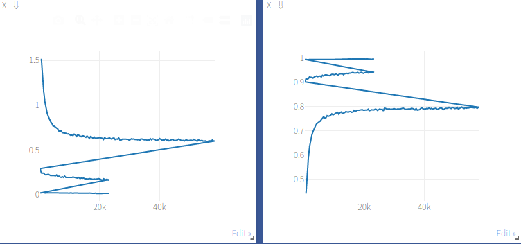
Test accuracy
---epoch57---
 25%|██▍       | 97/391 [00:03<00:08, 35.42it/s]epoch 57 iter 100 loss : 0.01788470149040222
 50%|█████     | 197/391 [00:05<00:05, 35.00it/s]Setting up a new session...
epoch 57 iter 200 loss : 0.019015971571207047
epoch 57 iter 200 train_acc : 0.9937499761581421
 77%|███████▋  | 301/391 [00:09<00:02, 32.77it/s]epoch 57 iter 300 loss : 0.01771947182714939
100%|██████████| 391/391 [00:11<00:00, 32.87it/s]
epoch 57 test_acc : 0.8694999814033508   Run a epoch Time spent: 12.92395305633545s
---epoch58---
 25%|██▍       | 97/391 [00:03<00:08, 33.84it/s]epoch 58 iter 100 loss : 0.01748574711382389
 50%|█████     | 197/391 [00:06<00:06, 32.05it/s]Setting up a new session...
epoch 58 iter 200 loss : 0.016185222193598747
epoch 58 iter 200 train_acc : 0.9952343702316284
 77%|███████▋  | 301/391 [00:09<00:02, 35.15it/s]epoch 58 iter 300 loss : 0.015332281589508057
100%|██████████| 391/391 [00:11<00:00, 33.29it/s]
epoch 58 test_acc : 0.8686999678611755   Run a epoch Time spent: 12.811056137084961s
---epoch59---
 26%|██▌       | 101/391 [00:03<00:08, 35.97it/s]epoch 59 iter 100 loss : 0.01672389917075634
 50%|█████     | 197/391 [00:05<00:05, 32.87it/s]Setting up a new session...
epoch 59 iter 200 loss : 0.0159761980175972
epoch 59 iter 200 train_acc : 0.9956249594688416
 76%|███████▌  | 297/391 [00:08<00:02, 35.49it/s]epoch 59 iter 300 loss : 0.016513127833604813
100%|██████████| 391/391 [00:11<00:00, 33.80it/s]
epoch 59 test_acc : 0.8678999543190002   Run a epoch Time spent: 12.58652377128601s

The process has ended with exit code 0
Summary of parameter adjustment
1. Add a weight attenuation to SGD, otherwise it will be over fitted, resulting in high training accuracy and low test accuracy.
2. Add another momentum and set the value to 0.9
 3. Adjust the parameter of weight attenuation to 5e-4
 4. Batch_ When the size is set to 128, the initial setting of 64 is not enough to make the model converge well
 5. When the training cannot converge well, you can add some more data enhancement
 6. In order to improve the training accuracy, the method of manually adjusting the learning rate is adopted. After 100 epochs, change the learning rate to 1e-3 and train 60 epochs
The parameters in this part refer to Pytorch actual combat 2: ResNet-18 realizes Cifar-10 image classification (the classification accuracy of test set is 95.170%)_ sunqiande88 blog - CSDN blog
I believe there are better trick or parameter adjustment for the classic model to improve the test accuracy. If you have better accuracy, please don't hesitate to leave a message in the comment area and tell me. Thank you!