Rent price analysis of rental housing in Shanghai
In this paper, we use crawler to crawl the housing rental data of Shanghai, and use python to clean, analyze and display the data, and carry out data mining modeling and prediction for housing rent.
# Import related packages
import pandas as pd
import numpy as np
import seaborn as sns
import matplotlib as mpl
import matplotlib.pyplot as plt
from IPython.display import display, Image

# Set the normal display of Chinese and negative sign
mpl.rcParams['font.sans-serif']=['SimHei']
mpl.rcParams['axes.unicode_minus']=False
sns.set_style({'font.sans-serif':['SimHei','Arial']})

%matplotlib inline
1, Reptile part
# Import related packages
import requests
from bs4 import BeautifulSoup
import json
import re
# Avoid anti pickpocketing and build headers and cookies. Otherwise, the website will detect illegal access request header information and return 404
# header
r_h = {'User-Agent': 'Mozilla/5.0 (Windows NT 10.0; Win64; x64; rv:76.0) Gecko/20100101 Firefox/76.0'}
# cookies
r_c = {}
cookies = '''F12 Check it on the Internet'''
for i in cookies.split('; '):
    r_c[i.split('=')[0]] = i.split('=')[1]

# Building crawler site infrastructure
district = ['jingan', 'xuhui', 'huangpu', 'changning', 'putuo', 'pudong',
            'baoshan', 'hongkou', 'yangpu', 'minhang', 'jinshan', 'jiading',
            'chongming', 'fengxian', 'songjiang', 'qingpu']
base_url = 'https://sh.zu.ke.com/zufang/'

# Find out how many pages of housing information each district has
district_info = {}
for i in district:
    pg_i = requests.get(url=base_url + i + '/', headers=r_h, cookies = r_c)
    pgsoup_i = BeautifulSoup(pg_i.text, 'lxml')
    num_i = pgsoup_i.find('div', class_ = "content__pg").attrs['data-totalpage']
    district_info[i] = int(num_i)

# Building a crawler website
url_list = []
for i, num in district_info.items():
    for j in range(1, num + 1):
        url_i = base_url + i + '/' + 'pg' + str(j) + '/'
        url_list.append(url_i)

# Crawling web information function
def data_request(urli, r_h, r_c):
    r_i = requests.get(url=urli, headers=r_h, cookies = r_c)
    soup_i = BeautifulSoup(r_i.text, 'lxml')
    div = soup_i.find('div', class_ = "content__list")
    info_list = div.find_all('div', class_ = "content__list--item--main")
    data_i = []
    for info in info_list:
        item = {}
        item['region'] = urli.split('/')[-3]
        item['info'] = info
        data_i.append(item)
    return data_i
# Crawling Web Information
data = []
for i in url_list:
    data.extend(data_request(i, r_h, r_c))
2, Data cleaning
# The data cleaning function is established to obtain the fields to be analyzed from crawling website information
def data_clear(data_i):
    item = {}
    item['region'] = data_i['region']
    info = data_i['info']
    item['house_info'] = ''.join(re.findall(r'\n\n\n(.+)\n\n\n', info.get_text())).replace(' ','')
    item['location_info'] = ''.join(re.findall(r'\n\n\n(.+)\n/\n', info.get_text())).replace(' ','')
    item['area_info'] = ''.join(re.findall(r'\n/\n(.+)㎡\n', info.get_text())).replace(' ','')
    item['floor_info'] = ''.join(re.findall(r'\n/\n(.+))\n', info.get_text())).replace(' ','').replace('(','')
    item['direction_info'] = ''.join(re.findall(r'\n(.+)/\n', info.get_text())).replace(' ','').replace('/','')
    item['layout_info'] = ''.join(re.findall(r'/\n(.+)\n/\n', info.get_text())).replace(' ','')
    item['price_info'] = ''.join(re.findall(r'\n\n(.+)element/month\n', info.get_text())).replace(' ','')
    item['other_info'] = ''.join(re.findall(r'\n                  \n\n\n([\s\S]*)\n\n', info.get_text())).replace(' ','')
    return item
# Data cleaning
data_c = []
for data_i in data:
    data_c.append(data_clear(data_i))
3, Data storage
# Import the related toolkit and establish the connection
import pymongo
myclient = pymongo.MongoClient("mongodb://localhost:27017/")
db = myclient['data']
beike_data = db['beike_data']
# Import data to mongodb
beike_data.insert_many(data_c)
# The normal acquisition process is to collect one and store one,
# Storage should be done in the data collection phase. This article is only to demonstrate the general usage of mongodb,
# Readers can try to save the data in the collection phase by themselves, and the method is consistent
<pymongo.results.InsertManyResult at 0x260c3179508>
# Simple data processing
data_pre = pd.read_csv("pd_data.csv",index_col=0)
# View the general structure of the data
data_pre[:3]

# Remove fields that are not related to the analysis
data_pre = data_pre.drop(['_id', 'region'], axis=1)
#
# View field data types
data_pre.info()
# OUTPUT
<class 'pandas.core.frame.DataFrame'>
Int64Index: 36622 entries, 0 to 36621
Data columns (total 8 columns):
area_info         36131 non-null object
direction_info    36499 non-null object
floor_info        34720 non-null object
house_info        36622 non-null object
layout_info       34729 non-null object
location_info     36131 non-null object
other_info        34720 non-null object
price_info        36622 non-null object
dtypes: object(8)
memory usage: 2.5+ MB
# Create an empty data frame
beike_df = pd.DataFrame()
# Extract fields
beike_df['Area'] = data_pre['area_info']
beike_df['Price'] = data_pre['price_info']
beike_df['Direction'] = data_pre['direction_info']
beike_df['Layout'] = data_pre['layout_info']
beike_df['Relative height'] = data_pre['floor_info'].str.split('floor', expand = True)[0]
beike_df['Total floors'] = data_pre['floor_info'].str.split('floor', expand = True)[1].str[:-1]
beike_df['Renting modes'] = data_pre['house_info'].str.split('·', expand = True)[0]
beike_df['District'] = data_pre['location_info'].str.split('-', expand = True)[0]
beike_df['Street'] = data_pre['location_info'].str.split('-', expand = True)[1]
beike_df['Community'] = data_pre['location_info'].str.split('-', expand = True)[2]
beike_df['Metro'] = data_pre['other_info'].str.contains('metro') + 0
beike_df['Decoration'] = data_pre['other_info'].str.contains('Hardcover') + 0
beike_df['Apartment'] = data_pre['other_info'].str.contains('apartment') + 0
# Data column position rearrangement is convenient to view and save to csv
columns = ['District', 'Street', 'Community', 'Renting modes','Layout', 'Total floors', 'Relative height', 'Area', 'Direction', 'Metro','Decoration', 'Apartment', 'Price']
df = pd.DataFrame(beike_df, columns = columns)
df.to_csv("df.csv",sep=',')
4, Add latitude and longitude geographic information field
# Construct the center point and take Shanghai International Hotel as the center point
center = (121.4671328,31.23570852)
# The location name column is exported separately and converted into longitude and latitude information by the third party platform
location_info = data_pre['location_info'].str.replace('-', '')
location_info.to_csv("location_info.csv",header='location',sep=',')
https://maplocation.sjfkai.com/ From this website, the geographic information points are transformed into corresponding longitude and latitude coordinates (Baidu coordinate system)
https://github.com/wandergis/coordTransform_py coordTransform_py module converts the latitude and longitude of Baidu coordinate system to wgs84
# Module description
# coord_converter.py [-h] -i INPUT -o OUTPUT -t TYPE [-n LNG_COLUMN] [-a LAT_COLUMN] [-s SKIP_INVALID_ROW]

# arguments:
#  -i , --input          Location of input file
#  -o , --output         Location of output file
#  -t , --type           Convert type, must be one of: g2b, b2g, w2g, g2w, b2w,
#                        w2b
#  -n , --lng_column     Column name for longitude (default: lng)
#  -a , --lat_column     Column name for latitude (default: lat)
#  -s , --skip_invalid_row
#                        Whether to skip invalid row (default: False)
# Read the geographic information of each point into pandas
geographic_info = pd.read_csv("wgs84.csv",index_col=0)
# Merge longitude and latitude
def point(x,y):
    return(x,y)
geographic_info['point'] = geographic_info.apply(lambda row:point(row['lat'],row['lng']),axis=1)
# geopy is used to calculate the distance between each point and the central point, as a field to reflect the degree of the rental location close to the city center
from geopy.distance import great_circle
center = (31.23570852,121.4671328)
list_d = []
for point in geographic_info['point']:
    list_d.append(great_circle(point, center).km)

geographic_info.insert(loc=4,column='distance',value=list_d
#
# Export to csv, reserve
geographic_info.to_csv("geographic_info.csv",sep=',')
5, Further data processing and Feature Engineering
df=pd.read_csv("df.csv",index_col=0)
#
# Check the data type and missing situation
df.info()
#
# OUTPUT
<class 'pandas.core.frame.DataFrame'>
Int64Index: 36622 entries, 0 to 36621
Data columns (total 13 columns):
District           36131 non-null object
Street             34728 non-null object
Community          34729 non-null object
Renting modes      36622 non-null object
Layout             34729 non-null object
Total floors       34712 non-null float64
Relative height    34720 non-null object
Area               36131 non-null object
Direction          36499 non-null object
Metro              34720 non-null float64
Decoration         34720 non-null float64
Apartment          34720 non-null float64
Price              36622 non-null object
dtypes: float64(4), object(9)
memory usage: 3.9+ MB***
There is a lot of information missing in the block and community of the house and the decoration of the house. Because the information can not be filled in, it will be removed later.
# View the data distribution of each field, mainly to clear invalid data (such as "unknown" and other unreasonable data)
df['District'].value_counts()
df['Street'].value_counts()
df['Community'].value_counts()
df['Renting modes'].value_counts()
df['Total floors'].value_counts()
df['Relative height'].value_counts()
df['Layout'].value_counts()
# Remove null value
df = df.dropna(how='any')
# Change the data type of the price and area fields to floating point
df[['Price','Area']] = df[['Price','Area']].astype(float)
# Change the field type of whether the subway has, decoration type and whether it is apartment to integer type
df[['Metro','Decoration','Apartment']] = df[['Metro','Decoration','Apartment']].astype(int)
# Remove the unknown data of house layout
df = df[~df['Layout'].str.contains("unknown")]
df.dtypes
# OUTPUT
District            object
Street              object
Community           object
Renting modes       object
Layout              object
Total floors       float64
Relative height     object
Area               float64
Direction           object
Metro                int32
Decoration           int32
Apartment            int32
Price              float64
dtype: object
- House orientation
# The house orientation is not in line with the common sense and needs to be cleaned up
df['Direction'].value_counts()
# OUTPUT
 South 25809
 North South 2956
 North 1980
 Southeast 835
 East 792
 West 534
 Southwest 499
 Northwest 217
 Southeast 202
 Northeast 160
 South southwest 69
 East east south south southwest West 66
 South West 57
 Things 41
 Southeast and North 36
 East southeast South North 35
 East Southeast 31
 South northwest 30
 Southeast and northwest 29
 East east south 21
 East southeast South West North South 19
 Southeast and southwest 15
 Southwest West 13
 Southeast South West north south 8
 South south 8
 West Northwest 7
 South West South West 6
 Southeast south southwest 6
 North northeast 5
 Southwest northeast 5
 Southeast and west 5
 South northeast 5
 Southwest northwest 5
 Southeast, north, South, north, northeast 5
 East West north 4
 South northwest North 4
 Southwest North 4
 South West north south 3
 Southeast South northwest 3
 East east south north 3
 North South northeast 3
 Southeast South northwest North 3
 Southwest West Northwest 3
 Southeast northeast 3
 Southeast South West 3
 East east south south northwest North 2
 East east south south southwest 2
 Northwest North 2
 East northeast 2
 Southeast southwest West Northwest northeast 1
 South southwest northwest 1
 South West Northwest North 1
 Southeast South West Northwest North 1
 Northeast 1
 Northwest northwest 1
 Northwest 1
Name: Direction, dtype: int64
# The main idea of building clean dictionary is to change the direction of repetition to simple type
cleanup_nums= {"Southeast South":"southeast","South southwest":"southwest","East east south south southwest West":"East West South",
               "nancy ":"southwest","East, Southeast, North and South":"Southeast and North","East Southeast":"southeast",
               "South Northwest":"Southwest and North","all directions":"the four corners of the world","East east south south":"southeast",
               "East, Southeast, South, West, North and South":"the four corners of the world","Southeast and southwest":"East West South","Southwest West":"southwest",
               "Southeast, South, West, North and South":"the four corners of the world","Southeast, South, North and South":"Southeast and North","west northwest":"northwest",
               "South West South West":"southwest","Southeast, South, Southwest":"East West South","Southwest and Northeast":"the four corners of the world",
               "Southwest Northwest":"Southwest and North","South Northeast":"Southeast and North","North northeast":"northeast",
               "Southeast, north, South, north, Northeast":"Southeast and North","Southeast and West":"East West South","South, northwest and North":"Southwest and North",
               "Southeast and Northeast":"Southeast and North","North South Northeast":"Southeast and North","East East South North":"Southeast and North",
               "Southeast South northwest North":"the four corners of the world","South West North South":"Southwest and North","Southwest West Northwest":"Southwest and North",
               "Southeast, South, Northwest":"the four corners of the world","Southeast, South and West":"East West South","Northeast China":"northeast",
               "Northwest North":"northwest","East east south south southwest":"East West South","East east south south northwest North":"the four corners of the world",
               "Southeast, South, West, northwest and North":"the four corners of the world","South West Northwest North":"Southwest and North","Northeast China":"northeast",
               "Southeast, southwest, West, northwest, Northeast":"the four corners of the world","South southwest Northwest":"Southwest and North","Northwest northwest North":"northwest",
               "Northwest China":"East West North"
              }
df['Direction'].replace(cleanup_nums,inplace=True)
# The above dictionary construction is too cumbersome, you can consider to do a duplicate, and then build the dictionary, which will save a lot of repetitive work.
#for i in len(df['Direction']):
#   df['Direction'][i] = ''.join(set(df['Direction'][i]))
#df['Direction']
#df['Direction'].value_counts()
#cleanup_nums can build fewer dictionaries
#df['Direction'].replace(cleanup_nums,inplace=True)
# House orientation information after cleaning
df['Direction'].value_counts()
# OUTPUT
 South 25809
 North South 2956
 North 1980
 Southeast 1089
 East 792
 Southwest 644
 West 534
 Northwest 227
 Northeast 168
 Southeast and North 98
 East West South 97
 East, West, North and South 71
 Southwest North 51
 Things 41
 East West North 5
Name: Direction, dtype: int64
- Housing area
df_aera = df['Area']
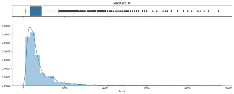
#sns histogram
f, (ax_box, ax_hist) = plt.subplots(2, sharex=True, gridspec_kw={"height_ratios": (.15, .85)}, figsize=(16, 10))
sns.boxplot(df_aera, ax=ax_box )
sns.distplot(df_aera, bins=40, ax=ax_hist)
# The abscissa of the box diagram is not displayed
ax_box.set(xlabel='')
ax_box.set_title('Housing area distribution')

The distribution of housing area is a long tail distribution, which does not meet the normal distribution of data modeling requirements. Here, we will simply deal with the following. The main processing idea is to remove the data with an area of more than 800 square meters but less than 6 square meters, which is obviously not of residential nature, and the data of more than 400 square meters but only one room is also removed.
df = df[(df['Area'] < 800)]
df = df[~(df['Area'] < 6)]
df = df[~((df['Area'] > 400) & (df['Layout'].str.contains('1 room')))]
df_aera = df['Area']
#sns histogram
f, (ax_box, ax_hist) = plt.subplots(2, sharex=True, gridspec_kw={"height_ratios": (.15, .85)},figsize=(16, 10))
sns.boxplot(df_aera, ax=ax_box)
sns.distplot(df_aera, bins=40, ax=ax_hist)
# Remove x axis name for the boxplot does not display the abscissa of the box plot
ax_box.set(xlabel='')
ax_box.set_title('Housing area distribution')

The data after cleaning is shown in the figure, which will be further processed.
- House price
f, ax_reg = plt.subplots(figsize=(16, 6))
sns.regplot(x='Area', y='Price', data=df, ax=ax_reg)
ax_reg.set_title('Relationship between housing area and price distribution')

After the preliminary cleaning up of the housing area, there will still be some outliers in the housing price, which will be cleaned up in the future, mainly to remove the data whose price is greater than 100000.
df_price = df['Price']

df = df[df['Price'] < 100000]
df_price = df['Price']
f, (ax_box, ax_hist) = plt.subplots(2, sharex=True, gridspec_kw={"height_ratios": (.15, .85)},figsize=(16, 6))
sns.boxplot(df_price, ax=ax_box)
sns.distplot(df_price, bins=40, ax=ax_hist)
# The abscissa of the box diagram is not displayed
ax_box.set(xlabel='')
ax_box.set_title('Housing area distribution')
f, ax_reg = plt.subplots(figsize=(16, 6))
sns.regplot(x='Area', y='Price', data=df, ax=ax_reg)
ax_reg.set_title('Relationship between housing area and price distribution')

There will still be some outliers, but the quality of the data is much better.
- Merge geographic information table with house information table
# Make connection fields
df['region'] = df['District'] + df['Street'] + df['Community']
geo=pd.read_csv("geographic_info.csv",index_col=0)
df_geo = pd.merge(df, geo, on='region', how='left')
# Remove analysis independent fields
df_geo = df_geo.drop(['region', 'point'], axis=1)
# Add the elevator field. There is no elevator information in the original data crawled. It is mainly judged by the total floor height. If the total floor is greater than 6 floors, there is an elevator
elevator = (df_geo['Total floors'] > 6) + 0
df_geo.insert(loc=4,column='Elevator',value=elevator)
# Export data
df_geo.to_csv("df_geo.csv", sep=',')
6, Data visualization
# The basic fields are visualized to understand the data distribution information and further process the data.
df_geo = pd.read_csv("df_geo.csv",index_col=0)
# The interactive visualization packages bokeh and pyecharts are used for visualization
# Import related packages
from bokeh.io import output_notebook
from bokeh.plotting import figure, show
from bokeh.models import ColumnDataSource
output_notebook()


import pyecharts.options as opts
from pyecharts.globals import ThemeType
from pyecharts.faker import Faker
from pyecharts.charts import Grid, Boxplot, Scatter, Pie, Bar
(https://bokeh.pydata.org)BokehJS 1.2.0 successfully loaded.
- Visualization of leasing mode
# Visualization of leasing mode
Renting_modes_group = df_geo.groupby('Renting modes')['Price'].count()
val = list(Renting_modes_group.astype('float64'))
var = list(Renting_modes_group.index)
p_group = (
    Pie(opts.InitOpts(width="1000px",height="600px",theme=ThemeType.LIGHT))
    .add("", [list(z) for z in zip(var, val)])
    .set_global_opts(title_opts=opts.TitleOpts(title="Rental form distribution"),
                 legend_opts=opts.LegendOpts(type_="scroll", pos_right="middle", orient="vertical"),
                 toolbox_opts=opts.ToolboxOpts())
    .set_series_opts(label_opts=opts.LabelOpts(formatter="{b}: {c}"))
)
p_group.render_notebook()

Among them, there are 5687 joint rent data. Because it is difficult to predict the whole rent of the house, it is not available to study the overall distribution of rent, and the proportion of joint rent in the total data is small. This analysis will remove the data, and a special topic can be opened to do the research on the distribution of joint rent in the future.
df_geo = df_geo[~(df_geo['Renting modes'] == 'Joint tenancy')]
- Geographic distance visualization
# The data 70 km away from the central point of Shanghai has exceeded the boundary of Shanghai City, which belongs to the error point generated by data processing, so remove it
df_geo = df_geo[~(df_geo['distance'] > 70)]
# The distance field is divided into 0-5, 5-10, 10-20, 20-70. The larger the number, the farther away from the city center.
bins = [0, 5, 10, 20, 70]
cats = pd.cut(df_geo.distance,bins)
df_geo['cats'] = cats

f, ax1 = plt.subplots(figsize=(16, 6))
sns.countplot(df_geo['cats'], ax=ax1, palette="husl")
ax1.set_title('Distribution of rental housing in different distance from the city center')

f, ax2 = plt.subplots(figsize=(16, 6))
sns.boxplot(x='cats', y='Price', data=df_geo, ax=ax2, palette="husl")
ax2.set_title('Price distribution of rental housing in different distances from the city center')

plt.show()


It can be seen from the figure that the number of rental houses within 5-10 km from the city center is the largest, followed by 0-5 km, and the number of houses in the more remote areas is relatively small, indicating that most people rent houses within 10 km from the city center. With the distance from the city center, the average price of rental housing is getting lower and lower. There is a gap of 2000 yuan between the average prices of each range.
- Visualization of house area
df_area = df_geo['Area']
df_price = df_geo['Area']
# bokeh histogram
hist, edge = np.histogram(df_area, bins=50)
p = figure(title="Area distribution of rental housing",plot_width=1000, plot_height=600, toolbar_location="above",tooltips="number: @top")
p.quad(top=hist, bottom=0, left=edge[:-1], right=edge[1:], line_color="white")

show(p)

#pyecharts histogram
hist, edge = np.histogram(df_area, bins=50)
x_data = list(edge[1:])
y_data = list(hist.astype('float64'))
bar = (
        Bar(init_opts = opts.InitOpts(width="1000px",height="600px",theme=ThemeType.LIGHT))
        .add_xaxis(xaxis_data=x_data)
        .add_yaxis("number", yaxis_data=y_data,category_gap=1)
        .set_global_opts(title_opts=opts.TitleOpts(title="Area distribution of rental housing"),
                        legend_opts=opts.LegendOpts(type_="scroll", pos_right="middle", orient="vertical"),
                        datazoom_opts=[opts.DataZoomOpts(type_="slider")], toolbox_opts=opts.ToolboxOpts(),
                        tooltip_opts=opts.TooltipOpts(is_show=True,axis_pointer_type= "line",trigger="item",formatter='{c}'))
        .set_series_opts(label_opts=opts.LabelOpts(is_show=False))
        )
bar.render_notebook()

The two interactive visualizations have many advantages over Seaborn, where you can click to see the number of each item and drag to see the range of interest.
- Rent price and quantity distribution of rental housing in urban areas
df_geo['Persq']=df_geo['Price']/df_geo['Area']
region_group_price = df_geo.groupby('District')['Price'].count().sort_values(ascending=False).to_frame().reset_index()
region_group_Persq = df_geo.groupby('District')['Persq'].mean().sort_values(ascending=False).to_frame().reset_index()
region_group = pd.merge(region_group_price, region_group_Persq, on='District')
x_region = list(region_group['District'])
y1_region = list(region_group['Price'].astype('float64'))
y2_region = list(region_group['Persq'])
bar_group = (
    Bar(opts.InitOpts(width="1000px",height="400px",theme=ThemeType.LIGHT))
    .add_xaxis(x_region)
    .add_yaxis("Num", y1_region, gap="5%")
    .add_yaxis("Persq", y2_region, gap="5%")
    .set_series_opts(label_opts=opts.LabelOpts(is_show=False))
    .set_global_opts(title_opts=opts.TitleOpts(title="The number of rental houses in each district and the rent price per unit area"),
                    legend_opts=opts.LegendOpts(type_="scroll", pos_right="middle", orient="vertical"),
                    datazoom_opts=[opts.DataZoomOpts(type_="slider")],
                    toolbox_opts=opts.ToolboxOpts(),
                    tooltip_opts=opts.TooltipOpts(is_show=True,axis_pointer_type= "line",trigger="item",formatter='{c}'))
    )
bar_group.render_notebook()

The number of rental housing and the rent price per unit area are similar to the distribution by region and distance. There are more rental houses in the central area, and the rent price per unit area is relatively high. The highest rent price per unit area is in Huangpu District, which is 158 yuan / square meter, and Chongming district is the lowest, which is 25 yuan / square meter.
region_group_price = df_geo.groupby('District')['Price']
box_data = []
for i in x_region:
    d = list(region_group_price.get_group(i))
    box_data.append(d)
# Rent price distribution of pyecharts districts
boxplot_group = Boxplot(opts.InitOpts(width="1000px",height="400px",theme=ThemeType.LIGHT))

boxplot_group.add_xaxis(x_region)
boxplot_group.add_yaxis("Price", boxplot_group.prepare_data(box_data))
boxplot_group.set_global_opts(title_opts=opts.TitleOpts(title="Rent price distribution in the upper districts"),
                        legend_opts=opts.LegendOpts(type_="scroll", pos_right="middle", orient="vertical"),
                        datazoom_opts=[opts.DataZoomOpts(),opts.DataZoomOpts(type_="slider")],
                        toolbox_opts=opts.ToolboxOpts(),
                        tooltip_opts=opts.TooltipOpts(is_show=True,axis_pointer_type= "line",trigger="item",formatter='{c}'))

boxplot_group.render_notebook()

# Rent price distribution of seaborn districts
f, ax = plt.subplots(figsize=(16,8))

sns.boxplot(x='District', y='Price', data=df_geo, palette="Set3", linewidth=2.5, order=x_region)
ax.set_title('Rent price distribution by district',fontsize=15)
ax.set_xlabel('region')
ax.set_ylabel('House rent')

plt.show()

According to the rent price distribution map of each district, Huangpu District still has the highest average rent price of rental housing, and there are abnormal points on the high side in each district. It is speculated that it should be the house type with more rooms such as villas. Songjiang, Jiading and Baoshan are located at a moderate distance from the city center, and their prices are lower than those in other districts. Therefore, they are suitable for office workers with lower budget.
- Orientation and type distribution of rental housing
f, ax1 = plt.subplots(figsize=(16,25))

sns.countplot(y='Layout', data=df_geo, ax=ax1,order = df_geo['Layout'].value_counts().index)
ax1.set_title('House type distribution',fontsize=15)
ax1.set_xlabel('number')
ax1.set_ylabel('House type')

f, ax2 = plt.subplots(figsize=(16,6))
sns.countplot(x='Direction', data=df_geo, ax=ax2,order = df_geo['Direction'].value_counts().index)
ax2.set_title('House orientation distribution',fontsize=15)
ax2.set_xlabel('orientation')
ax2.set_ylabel('number')


plt.show()


Among the house types, small ones account for a large proportion, while those with multiple rooms account for a relatively small proportion. Among them, the type of one room, one hall and one bathroom is the most, which is also in line with the trend that many people want to have their own private space, followed by two rooms and one hall. Most of the houses face south, which is in line with the common sense of architectural design. The remaining north-south composite orientation should be the superposition of different room orientations, and the number of houses with South orientation is still the largest.
- Relationship between rental price and elevator, subway, decoration and apartment fields
sns.catplot(x='Elevator',y='Price',hue='Metro',row='Apartment',
            col='Decoration',data=df_geo,kind="box",palette="husl")

The rental price of houses with elevators is generally higher than that of houses without elevators, and the same factor of subway also makes housing rents higher. In most cases, the rental price of hardcover housing is high, and whether it is the apartment has no regular effect on the rent price of housing.
- Relationship between rental price and floor height of rental housing
f, ax1 = plt.subplots(figsize=(16, 4))
sns.countplot(df_geo['Relative height'], ax=ax1, palette="husl")
ax1.set_title('Number distribution of rental housing with different storey height')
f, ax2 = plt.subplots(figsize=(16, 8))
sns.boxplot(x='Relative height', y='Price', data=df_geo, ax=ax2, palette="husl")
ax2.set_title('Rent price distribution of rental housing with different storey height')
plt.show()


The number of rental rooms in medium height floor is the most, and that of low floor is the least. On the contrary, the average rental price of low floor is the highest, while that of high floor is the lowest, which is supposed to be due to the higher living convenience of low floor.
- Thermal map of rent price distribution of rental housing in different districts
# Import related modules
from pyecharts.charts import Geo
from pyecharts.globals import ChartType
from pyecharts.globals import GeoType
# Construct data set
region = df_geo['District'] + df_geo['Street'] + df_geo['Community']
region = region.reset_index(drop=True)
data_pair = [(region[i], df_geo.iloc[i]['Price']) for i in range(len(region))]
pieces=[
      {'max': 1000,'label': '1000 following','color':'#50A3BA'},  #There is an upper limit but no lower limit, and the label and color are customized
      {'min': 1000, 'max': 1800,'label': '1000-1800','color':'#81AE9F'},
      {'min': 1800, 'max': 2300,'label': '1800-2300','color':'#E2C568'},
      {'min': 2300, 'max': 2800,'label': '2300-2800','color':'#FCF84D'},
      {'min': 2800, 'max': 5000,'label': '2800-5000','color':'#E49A61'},
      {'min': 5000, 'max': 8000,'label': '5000-8000','color':'#DD675E'},
      {'min': 8000, 'label': '8000 above','color':'#D94E5D'}#There is a lower limit but no upper limit
]
# Thermal map of rent price distribution of rental housing in different districts
geo = Geo(opts.InitOpts(width="600px",height="600px",theme=ThemeType.LIGHT))
geo.add_schema(maptype = "Shanghai",emphasis_label_opts=opts.LabelOpts(is_show=True,font_size=16))
for i in range(len(region)):
    geo.add_coordinate(region[i],df_geo.iloc[i]['lng'],df_geo.iloc[i]['lat'])
geo.add("",data_pair,type_=GeoType.HEATMAP)
geo.set_global_opts(
                    title_opts=opts.TitleOpts(title="Rent distribution in Shanghai"),
                    visualmap_opts=opts.VisualMapOpts(min_ = 0,max_ = 30000,split_number = 20,range_text=["High", "Low"],is_calculable=True,range_color=["lightskyblue", "yellow", "orangered"]),
                    toolbox_opts=opts.ToolboxOpts(),
                    tooltip_opts=opts.TooltipOpts(is_show=True)
                  )
geo.set_series_opts(label_opts=opts.LabelOpts(is_show=False))
geo.render_notebook()
#geo.render("HEATMAP.html")

The thermal chart of house rent price reflects the level of rent and the density of houses in a region. The display effect of the thermal chart made by pyechards is not very good. Therefore, it uses pyechards to make a scatter chart of price distribution as a supplement. The two graphs express the same meaning. Later, it is exported to tableau for a version, and the display effect is better than that of pyechharts.
# Scatter chart of rental price distribution in different districts
geo = Geo(opts.InitOpts(width="600px",height="600px",theme=ThemeType.LIGHT))
geo.add_schema(maptype = "Shanghai")
for i in range(len(region)):
    geo.add_coordinate(region[i],df_geo.iloc[i]['lng'],df_geo.iloc[i]['lat'])
geo.add("",data_pair,type_=GeoType.EFFECT_SCATTER,symbol_size=5)
geo.set_global_opts(
                    title_opts=opts.TitleOpts(title="Rent distribution in Shanghai"),
                    visualmap_opts=opts.VisualMapOpts(is_piecewise=True, pieces=pieces),
                    toolbox_opts=opts.ToolboxOpts()
                  )
geo.set_series_opts(label_opts=opts.LabelOpts(is_show=False))
geo.render_notebook()
#geo.render("SCATTER.html")

7, Data modeling
- Feature Engineering
# Read data
data=pd.read_csv("df_geo_df.csv",index_col=0)
# Remove modeling independent features
data = data.drop(['Street', 'Community', 'Renting modes', 'Total floors', 'lng', 'lat', 'cats', 'Persq'], axis=1)
# The Distance field is a continuous variable, which is removed after discretization.
bins = [0, 5, 10, 20, 70]
cats = pd.cut(data.distance,bins)
data['cats'] = cats
data = data.drop(['distance'], axis=1)
If every different Year value is taken as the characteristic value, we can not find out the influence of Year on Price, because the division of years is too detailed. Therefore, we have to discretize the continuous numerical feature Year and do the box processing. After feature discretization, the model will be more stable and reduce the risk of model over fitting.
# The feature of house layout can not be directly used as model input, and the number of rooms, halls and toilets can be extracted from it
data['room_num'] =  data['Layout'].str.extract('(^\d).*', expand=False).astype('int64')
data['hall_num'] =   data['Layout'].str.extract('^\d.*?(\d).*', expand=False).astype('int64')
data['bathroom_num'] =  data['Layout'].str.extract('^\d.*?\d.*?(\d).*', expand=False).astype('int64')
#The data in this paper are relatively regular, which can be directly. STR [0]. STR [2]. STR [4]
# Create a new feature
# The main idea is to consider the shared living area, hall and toilet shared by each tenant,
# A new field "convenience" is generated to represent the living comfort. The larger the value, the higher the living comfort
data['area_per_capita'] = data['Area'] / data['room_num']
data['area_per_capita_norm'] = data[['area_per_capita']].apply(lambda x: (x - np.min(x)) / (np.max(x) - np.min(x)))
data['convenience'] = data['area_per_capita_norm'] + (data['hall_num'] / data['room_num']) + (data['bathroom_num'] / data['room_num'])
# Remove modeling independent features
data = data.drop(['Layout', 'area_per_capita', 'area_per_capita_norm'], axis=1)
# Reset index
data = data.reset_index(drop = True)
# The feature data of region, relative height and orientation are changed from Chinese to abbreviation
district_nums = {"Jiading":"JD","Fengxian":"FX","Baoshan":"BS","Chongming":"CM",
                 "Xuhui":"XH","Putuo":"PT","Yangpu":"YP","Songjiang":"SJ",
                 "Pudong":"PD","Hongkou":"HK","Jinshan":"JS","Changning":"CN",
                 "Minhang":"MH","Qingpu":"QP","Jing'an":"JA","Huangpu":"HP"}
relative_height_nums = {"high":"H","in":"M","low":"L"}
direction_nums = {"east":"E","northeast":"EN","southeast":"ES","Southeast and North":"ESN",
                  "thing":"EW","East West North":"EWN","East West South":"EWS",
                  "the four corners of the world":"EWSN","north":"N","south":"S","north and south":"SN",
                  "west":"W","northwest":"WN","southwest":"WS","Southwest and North":"WSN"}
data['District'].replace(district_nums,inplace=True)
data['Relative height'].replace(relative_height_nums,inplace=True)
data['Direction'].replace(direction_nums,inplace=True)
# Repeat name section name
data_columns = {"Relative height":"rh","cats":"distance_cat"}
data.rename(columns = data_columns,inplace = True)
data.columns = data.columns.str.lower()
# Finally, check whether the data type of each field is reasonable
data.info()
# OUTPUT
<class 'pandas.core.frame.DataFrame'>
RangeIndex: 28799 entries, 0 to 28798
Data columns (total 14 columns):
district        28799 non-null object
elevator        28799 non-null int64
rh              28799 non-null object
area            28799 non-null float64
direction       28799 non-null object
metro           28799 non-null int64
decoration      28799 non-null int64
apartment       28799 non-null int64
price           28799 non-null float64
distance_cat    28733 non-null category
room_num        28799 non-null int64
hall_num        28799 non-null int64
bathroom_num    28799 non-null int64
convenience     28799 non-null float64
dtypes: category(1), float64(3), int64(7), object(3)
memory usage: 2.9+ MB
# Reorder the columns of the dataset for easy viewing
data_order = ['price','area','convenience','district','elevator','rh',
              'direction','metro','decoration','apartment','distance_cat',
              'room_num','hall_num','bathroom_num' ]
data = data[data_order]
# Take out the characteristics of numerical type for visualization
numeric_dtypes = ['int16', 'int32', 'int64', 'float16', 'float32', 'float64']
numeric = []
for i in data.columns:
    if data[i].dtype in numeric_dtypes:
        if i in ['elevator','metro','decoration','apartment']:
            pass
        else:
            numeric.append(i)
# Visualization of numerical data
f, ax = plt.subplots(figsize=(14, 6))
ax.set_xscale("log")
ax = sns.boxplot(data=data[numeric], orient="h", palette="husl")
ax.xaxis.grid(False)
ax.set(ylabel="Names")
ax.set(xlabel="Values")
ax.set(title="Data Distribution")
for tick in ax.xaxis.get_major_ticks():
        tick.label1.set_fontproperties('stixgeneral')

# Rectification
from scipy.stats import skew, norm
from scipy.special import boxcox1p
from scipy.stats import boxcox_normmax
# Find out the skew data
skew_col = data[numeric].apply(lambda x: skew(x))
high_skew = skew_col[skew_col > 0.5]
high_skew_index = high_skew.index
high_skew_index = high_skew_index.drop('price')
# Rectification
data['price'] = np.log1p(data['price'])
for i in high_skew_index:
    data[i] = boxcox1p(data[i], boxcox_normmax(data[i] + 1))
# Distribution of numerical data after rectification
f, ax = plt.subplots(figsize=(14, 6))
ax.set_xscale("log")
ax = sns.boxplot(data=data[numeric], orient="h", palette="husl")
ax.xaxis.grid(False)
ax.set(ylabel="Names")
ax.set(xlabel="Values")
ax.set(title="Data Distribution")
for tick in ax.xaxis.get_major_ticks():
        tick.label1.set_fontproperties('stixgeneral')

# Take out the area and price to see the data distribution
cols = ['area','price']
fig, axs = plt.subplots(ncols=1, nrows=0, figsize=(14, 14))
plt.subplots_adjust(right=1)
plt.subplots_adjust(top=1)
sns.color_palette("husl")

for i, col in enumerate(cols, 1):
    plt.subplot(len(cols), 2, i)
    sns.distplot(data[col], bins=30)
    plt.xlabel('{}'.format(col), size=15,labelpad=12.5)
    for j in range(2):
        plt.tick_params(axis='x', labelsize=12)
        plt.tick_params(axis='y', labelsize=12)

plt.show()

Area and price characteristics are basically normal distribution after processing
# For the features such as region and orientation that can not be used as model input, these non numerical values need to be quantized. The processing method is to use the single heat code and process it as 01 format.
for cols in data.columns:
    if (data[cols].dtype == np.object) or (cols == 'distance_cat'):
        data = pd.concat((data, pd.get_dummies(data[cols], prefix=cols, dtype=np.int64)), axis=1)
        del data[cols]
data.info()
# OUTPUT
<class 'pandas.core.frame.DataFrame'>
RangeIndex: 28799 entries, 0 to 28798
Data columns (total 48 columns):
price                    28799 non-null float64
area                     28799 non-null float64
convenience              28799 non-null float64
elevator                 28799 non-null int64
metro                    28799 non-null int64
decoration               28799 non-null int64
apartment                28799 non-null int64
room_num                 28799 non-null float64
hall_num                 28799 non-null int64
bathroom_num             28799 non-null float64
district_BS              28799 non-null int64
district_CM              28799 non-null int64
district_CN              28799 non-null int64
district_FX              28799 non-null int64
district_HK              28799 non-null int64
district_HP              28799 non-null int64
district_JA              28799 non-null int64
district_JD              28799 non-null int64
district_JS              28799 non-null int64
district_MH              28799 non-null int64
district_PD              28799 non-null int64
district_PT              28799 non-null int64
district_QP              28799 non-null int64
district_SJ              28799 non-null int64
district_XH              28799 non-null int64
district_YP              28799 non-null int64
rh_H                     28799 non-null int64
rh_L                     28799 non-null int64
rh_M                     28799 non-null int64
direction_E              28799 non-null int64
direction_EN             28799 non-null int64
direction_ES             28799 non-null int64
direction_ESN            28799 non-null int64
direction_EW             28799 non-null int64
direction_EWN            28799 non-null int64
direction_EWS            28799 non-null int64
direction_EWSN           28799 non-null int64
direction_N              28799 non-null int64
direction_S              28799 non-null int64
direction_SN             28799 non-null int64
direction_W              28799 non-null int64
direction_WN             28799 non-null int64
direction_WS             28799 non-null int64
direction_WSN            28799 non-null int64
distance_cat_(0, 5]      28799 non-null int64
distance_cat_(5, 10]     28799 non-null int64
distance_cat_(10, 20]    28799 non-null int64
distance_cat_(20, 70]    28799 non-null int64
dtypes: float64(5), int64(43)
memory usage: 10.5 MB
data.shape
# OUTPUT
(28799, 48)
# Visualization of feature correlation
colormap = plt.cm.OrRd
plt.figure(figsize=(40,40))
sns.heatmap(data.corr(),cbar=True,linewidths=0.1,vmax=1.0, square=True,
            fmt='.2f',cmap=colormap, linecolor='white', annot=True)

# Data export backup
data.to_csv("all_data.csv", sep=',')
all_data=pd.read_csv("all_data.csv",index_col=0)
- model training
# Import related packages
# This project uses decision tree with pruning to train the model
from sklearn.model_selection import KFold
from sklearn.ensemble import RandomForestRegressor
from sklearn.metrics import make_scorer, mean_squared_error
from sklearn.model_selection import GridSearchCV
from sklearn.pipeline import make_pipeline


from sklearn.model_selection import learning_curve, validation_curve
from sklearn.model_selection import cross_val_score
from sklearn.metrics import r2_score
from sklearn.model_selection import ShuffleSplit
plt.style.use('bmh')

import warnings
warnings.filterwarnings(action="ignore")
# Creating feature sets
X = all_data.drop('price', axis=1)
X.shape
# OUTPUT
(28799, 47)
# Create label set
y = all_data['price']
y.shape
# OUTPUT
(28799,)
#Under different model parameters, the learning curve shows the change of model training set score and verification set score with the increase of training data,
#This paper focuses on the performance of decision tree model under different maximum depths.
# r2_score: the percentage of the square of the correlation degree between the predicted value and the actual value of the target variable. The numerical value represents the percentage of the target variable in the model that can be explained by the characteristics

#When all data sets are trained, the score of model training set and verification set changes with the change of model parameters,
#This time, we focus on the performance of decision tree model under different maximum depths.

From the learning curve, with the increase of training data, the score of training set decreases, while the score of verification set increases. When the amount of data reaches a certain scale, the scores of training set and verification set tend to be stable, and then the increase of data volume can not improve the performance of the model. When the maximum depth of the model is 11, the deviation and variance of the model prediction reach equilibrium. From the complexity curve, when the maximum depth is greater than 11, the score of model validation set decreases steadily, and the variance becomes larger and larger, and the trend of fitting has appeared. Combined with the results of the two curves, it is considered that the maximum depth of the model is 11 and the prediction effect is the best.
# Divide training set and test set
from sklearn.model_selection import train_test_split
X_train, X_test, y_train, y_test = train_test_split(X, y, test_size=0.2, random_state=42)
# Grid search is used to find the best combination of parameters
# The score of each parameter combination is obtained by cross validation to determine the optimal parameter combination

# Value range of optimization parameters
param_grid = {
    'max_depth': list(range(6, 16)),
    'min_samples_split': [70, 80, 90],
    'max_features': [8, 10, 12],
    'min_samples_leaf':[14, 16, 18]
    }
# Cross validation
cv = ShuffleSplit(n_splits = 10, test_size = 0.2, random_state = 0)
# Define training model
rf = RandomForestRegressor(random_state=42)
# Grid search
grid_search = GridSearchCV(estimator = rf, param_grid = param_grid,
                           scoring='r2', cv = cv, n_jobs = 4, verbose = 1)
grid_search.fit(X_train, y_train)
# Optimal parameters
grid_search.best_params_
# OUTPUT
{'max_depth': 14,
 'max_features': 12,
 'min_samples_leaf': 14,
 'min_samples_split': 70}
# Scoring function
def evaluate(model, test_features, test_labels):
    predictions = model.predict(test_features)
    score = r2_score(test_labels, predictions)
    print('R2_score = {:0.4f}'.format(score))
# The data set was trained and scored with the optimal parameters
best_grid = grid_search.best_estimator_
evaluate(best_grid, X_test, y_test)
# OUTPUT
R2_score = 0.8828
Improvement: try to use a variety of regression models for prediction, compare the calculation efficiency and accuracy, try to model fusion. Add new fields in the data set, such as: the living convenience of the surrounding areas, more subdivision of the decoration status (hardcover and simple decoration blank), the year of building completion, whether the water and electricity are civil, whether the supporting facilities are complete, etc.