The relationship between variable and option price in BS formula
according to BS formula, we know that there are five variables that jointly affect the option price: S, K, r, σ and t. let'S draw a picture to directly feel the relationship between these variables and the call put option price. Using the data from the last example in the previous section, S, K, r, σ and T are 5.29, 6, 0.04, 0.24 and 0.5, respectively
from scipy.stats import norm
import numpy as np
def bscall(S,K,r,sigma,t):
	d1=(np.log(S/K)+(r+0.5*sigma**2)*t)/(sigma*np.sqrt(t))
	d2=(np.log(S/K)+(r-0.5*sigma**2)*t)/(sigma*np.sqrt(t))
	return S*norm.cdf(d1)-K*np.exp(-r*t)*norm.cdf(d2)
def bsput(S,K,r,sigma,t):
	d1=(np.log(S/K)+(r+0.5*sigma**2)*t)/(sigma*np.sqrt(t))
	d2=(np.log(S/K)+(r-0.5*sigma**2)*t)/(sigma*np.sqrt(t))
	return -S*norm.cdf(-d1)+K*np.exp(-r*t)*norm.cdf(-d2)

import matplotlib.pyplot as plt
from pylab import mpl
mpl.rcParams['font.sans-serif']=['SimHei']
mpl.rcParams['axes.unicode_minus']=False
plt.figure(figsize=(18,12))
plt.subplot(231)
S=np.linspace(3,7,100)
plt.plot(S,bscall(S,6,0.04,0.24,0.5),'r-',label='Call option')
plt.plot(S,bsput(S,6,0.04,0.24,0.5),'k-',label='Put option')
plt.xlabel('Share price')
plt.ylabel('Option price')
plt.title('The relationship between stock price and option price')
plt.legend()
plt.subplot(232)
K=np.linspace(5,7,100)
plt.plot(K,bscall(5.29,K,0.04,0.24,0.5),'r-',label='Call option')
plt.plot(K,bsput(5.29,K,0.04,0.24,0.5),'k-',label='Put option')
plt.xlabel('Execution price')
plt.ylabel('Option price')
plt.title('Relationship between execution price and option price')
plt.legend()
plt.subplot(233)
sigma=np.linspace(0.1,0.4,100)
plt.plot(sigma,bscall(5.29,6,0.04,sigma,0.5),'r-',label='Call option')
plt.plot(sigma,bsput(5.29,6,0.04,sigma,0.5),'k-',label='Put option')
plt.xlabel('Volatility')
plt.ylabel('Option price')
plt.title('The relationship between volatility and option price')
plt.legend()
plt.subplot(234)
r=np.linspace(0.01,0.07,100)
plt.plot(r,bscall(5.29,6,r,0.24,0.5),'r-',label='Call option')
plt.plot(r,bsput(5.29,6,r,0.24,0.5),'k-',label='Put option')
plt.xlabel('Risk free rate of return')
plt.ylabel('Option price')
plt.title('The relationship between risk-free rate of return and option price')
plt.legend()
plt.subplot(235)
t=np.linspace(0,3,500)
plt.plot(t,bscall(5.29,6,0.04,0.24,t),'r-',label='Call option')
plt.plot(t,bsput(5.29,6,0.04,0.24,t),'k-',label='Put option')
plt.xlabel('Maturity')
plt.ylabel('Option price')
plt.title('Relationship between maturity and option price')
plt.legend()
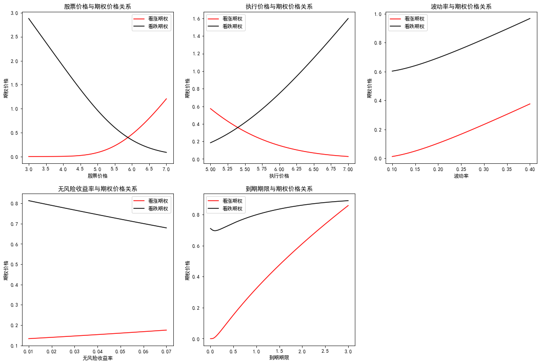
the relationship between the option price and the stock price S and the execution price k is easy to understand; the call put option is directly proportional to the volatility σ because the volatility reflects the time value of the option, and the time value for the option buyer reflects the possibility that the intrinsic value of the option will increase in the future; when the risk-free interest rate r increases, the call option price increases, and the put option price decreases because R The increase of the discount rate means that the discount rate will also increase, resulting in the decrease of the present value of K. at the same time, the opportunity cost of holding the basic assets in the hands of high interest rate is also higher, so the decrease of the value of put option is larger than the increase of call option. The direct ratio between the maturity and the value of option is also related to the value of time, but there may be exceptions when the option expires immediately, such as deep in the- Money put, the longer the waiting time is, the worse for the holder.
Measuring option risk with Greek value
Delta
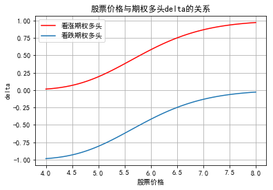
. The delta of European call options and put options (long) are △ = N(d1), △ = N(d1)-1 respectively, and the short ones are all added with a negative sign. Here's a picture of the relationship between the ∆ of option bull and stock price:
def delta(S,X,r,sigma,t,otype):
	d1=(np.log(S/X)+(r+0.5*sigma**2)*t)/(sigma*np.sqrt(t))
	if otype=='call':
		return norm.cdf(d1)
	else:
		return norm.cdf(d1)-1
S1=np.linspace(4,8,100)
plt.plot(S1,delta(S1,6,0.04,0.24,0.5,'call'),'r-',label='buy a call ')
plt.plot(S1,delta(S1,6,0.04,0.24,0.5,'put'),label='long put option ')
plt.xlabel('Share price')
plt.ylabel('delta')
plt.title('Stock price and option bull delta Relationship')
plt.legend()
plt.grid()
Q Q Q .
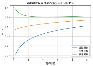
T=np.linspace(0,5,100)
plt.plot(T,delta(5,6,0.04,0.24,T,'call'),label='Virtual option')
plt.plot(T,delta(6,6,0.04,0.24,T,'call'),label='Flat option')
plt.plot(T,delta(7,6,0.04,0.24,T,'call'),label='Real options')
plt.xlabel('Maturity')
plt.ylabel('delta')
plt.title('Maturity and call option bull delta Relationship')
plt.legend()
plt.grid()
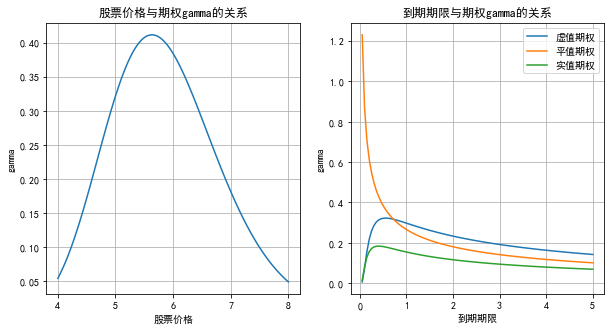
Gamma
. According to the second derivative of BS formula, the Gamma expressions of European call and put options are as follows: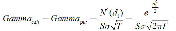
def gamma(S,X,r,sigma,t):
	d1=(np.log(S/X)+(r+0.5*sigma**2)*t)/(sigma*np.sqrt(t))
	return np.exp(-d1**2/2)/(S*sigma*np.sqrt(2*np.pi*t))
plt.figure(figsize=(10,5))
plt.subplot(121)
plt.plot(S1,gamma(S1,6,0.04,0.24,0.5))
plt.xlabel('Share price')
plt.ylabel('gamma')
plt.title('Stock price and options gamma Relationship')
plt.grid()
plt.subplot(122)
plt.plot(T,gamma(5,6,0.04,0.24,T),label='Virtual option')
plt.plot(T,gamma(6,6,0.04,0.24,T),label='Flat option')
plt.plot(T,gamma(7,6,0.04,0.24,T),label='Real options')
plt.xlabel('Maturity')
plt.ylabel('gamma')
plt.title('Maturity and options gamma Relationship')
plt.legend()
plt.grid()
.
Theta
. That is to say, the change of the right price in a unit period with a shorter period of validity, and the first derivative of the option price to the period of validity.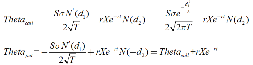
def theta(S,X,r,sigma,t,otype):
	d1=(np.log(S/X)+(r+0.5*sigma**2)*t)/(sigma*np.sqrt(t))
	d2=(np.log(S/K)+(r-0.5*sigma**2)*t)/(sigma*np.sqrt(t))
	thetac=-S*sigma*np.exp(-d1**2/2)/(2*np.sqrt(2*np.pi*t))-r*X*np.exp(-r*t)*norm.cdf(d2)
	if otype=='call':
		return thetac
	else:
		return thetac+r*X*np.exp(-r*t)
plt.figure(figsize=(10,5))
plt.subplot(121)
plt.plot(S1,theta(S1,6,0.04,0.24,0.5,'call'),label='Call option')
plt.plot(S1,theta(S1,6,0.04,0.24,0.5,'put'),label='Put option')
plt.xlabel('Share price')
plt.ylabel('theta')
plt.title('Stock price and options theta Relationship')
plt.legend()
plt.grid()
plt.subplot(122)
plt.plot(T,theta(5,6,0.04,0.24,T,'call'),label='Virtual option')
plt.plot(T,theta(6,6,0.04,0.24,T,'call'),label='Flat option')
plt.plot(T,theta(7,6,0.04,0.24,T,'call'),label='Real options')
plt.xlabel('Maturity')
plt.ylabel('theta')
plt.title('Maturity and call options theta Relationship')
plt.legend()
plt.grid()

it can be seen from the above figure that θ is negative and the.
Vega
.
Similarly, we can draw the relationship between vega and stock price, and the relationship between vega and option maturity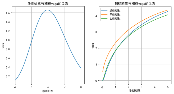
.
Rho
.
draw the relationship between rho and stock price, as well as the relationship between rho and option maturity: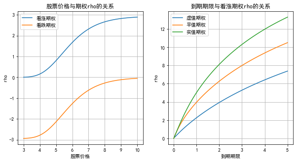
.

