Warm tip: this case is only for learning and research purposes, and does not constitute an investment proposal.

The price data of bitcoin is based on time series, so the price prediction of bitcoin is mostly realized by LSTM model.

Long term short-term memory (LSTM) is a kind of deep learning model especially suitable for time series data (or data with time / space / structure order, such as movies, sentences, etc.), which is an ideal model to predict the price trend of cryptocurrencies.

In this paper, we mainly write data fitting through LSTM to predict the future price of bitcoin.

Libraries needed for import

import pandas as pd
import numpy as np

from sklearn.preprocessing import MinMaxScaler, LabelEncoder
from keras.models import Sequential
from keras.layers import LSTM, Dense, Dropout

from matplotlib import pyplot as plt
%matplotlib inline

Data analysis

Data loading

Read daily transaction data of BTC

data = pd.read_csv(filepath_or_buffer="btc_data_day")

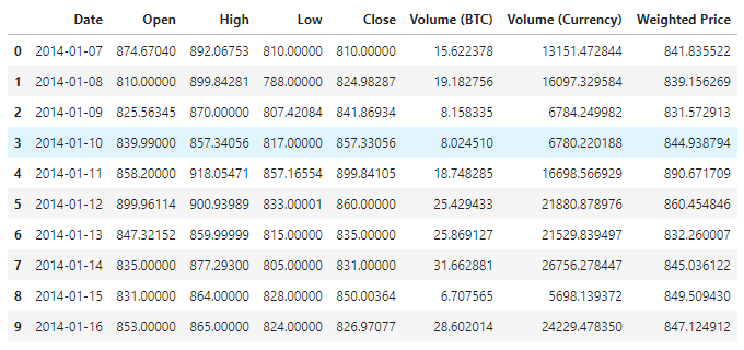
You can get 1380 pieces of data by viewing the data. The data consists of Date, Open, High, Low, Close, Volume(BTC), Volume(Currency) and Weighted Price. Except for the Date column, the rest of the data columns are of the float64 data type.

data.info()

View the data in the first 10 rows

data.head(10)

Data visualization

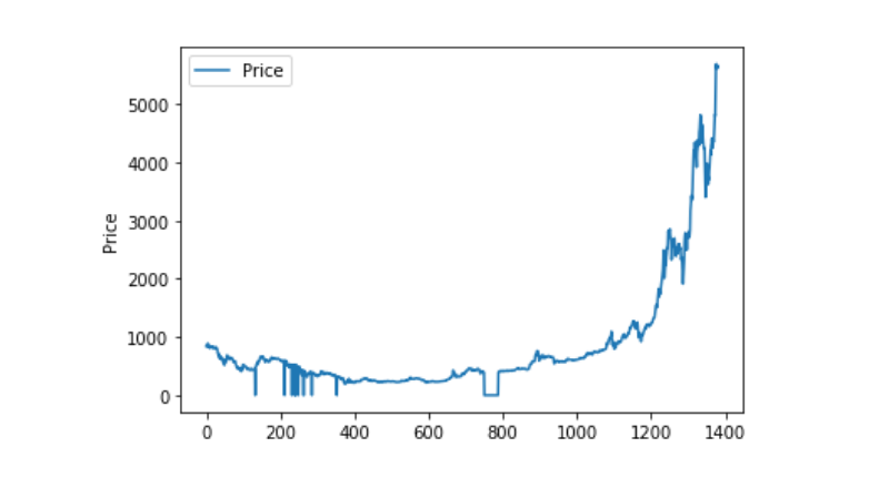
Use matplotlib to draw Weighted Price to see the distribution and trend of data. In the figure, we found that there is a section of data 0. We need to confirm whether the data is abnormal.

plt.plot(data['Weighted Price'], label='Price')
plt.ylabel('Price')
plt.legend()
plt.show()

Abnormal data processing

First, check whether the data contains nan data. You can see that there is no nan data in our data

data.isnull().sum()

Date                 0
Open                 0
High                 0
Low                  0
Close                0
Volume (BTC)         0
Volume (Currency)    0
Weighted Price       0
dtype: int64

Look at the 0 data again. You can see that our data contains 0 value. We need to process the 0 value

(data == 0).astype(int).any()

Date                 False
Open                  True
High                  True
Low                   True
Close                 True
Volume (BTC)          True
Volume (Currency)     True
Weighted Price        True
dtype: bool

data['Weighted Price'].replace(0, np.nan, inplace=True)
data['Weighted Price'].fillna(method='ffill', inplace=True)
data['Open'].replace(0, np.nan, inplace=True)
data['Open'].fillna(method='ffill', inplace=True)
data['High'].replace(0, np.nan, inplace=True)
data['High'].fillna(method='ffill', inplace=True)
data['Low'].replace(0, np.nan, inplace=True)
data['Low'].fillna(method='ffill', inplace=True)
data['Close'].replace(0, np.nan, inplace=True)
data['Close'].fillna(method='ffill', inplace=True)
data['Volume (BTC)'].replace(0, np.nan, inplace=True)
data['Volume (BTC)'].fillna(method='ffill', inplace=True)
data['Volume (Currency)'].replace(0, np.nan, inplace=True)
data['Volume (Currency)'].fillna(method='ffill', inplace=True)

(data == 0).astype(int).any()

Date                 False
Open                 False
High                 False
Low                  False
Close                False
Volume (BTC)         False
Volume (Currency)    False
Weighted Price       False
dtype: bool

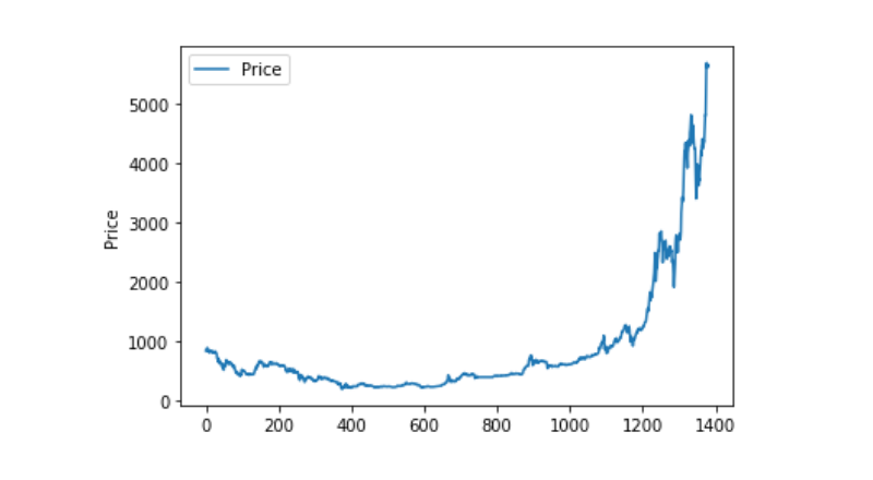
Look at the distribution and trend of the data. At this time, the curve is very continuous

plt.plot(data['Weighted Price'], label='Price')
plt.ylabel('Price')
plt.legend()
plt.show()

Partition of training data set and test data set

Normalize data to 0-1

data_set = data.drop('Date', axis=1).values
data_set = data_set.astype('float32')
mms = MinMaxScaler(feature_range=(0, 1))
data_set = mms.fit_transform(data_set)

Divide test data set and training data set by 2:8

ratio = 0.8
train_size = int(len(data_set) * ratio)
test_size = len(data_set) - train_size
train, test = data_set[0:train_size,:], data_set[train_size:len(data_set),:]

Create training data set and test data set, and use 1 day as window period to create our training data set and test data set.

def create_dataset(data):
    window = 1
    label_index = 6
    x, y = [], []
    for i in range(len(data) - window):
        x.append(data[i:(i + window), :])
        y.append(data[i + window, label_index])
    return np.array(x), np.array(y)

train_x, train_y = create_dataset(train)
test_x, test_y = create_dataset(test)

Define model and train

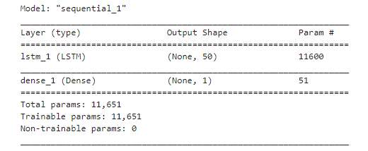
This time we use a simple model. The structure of this model is as follows: 1. LSTM2. Dense.

Here we need to explain the Input Shape of LSTM. The input dimension of Input Shape is (batch_size, time steps, features). Where, the time steps value is the time window interval when data is input. Here we use 1 day as the time window, and our data is daily data, so our time steps here is 1.

Long short term memory (LSTM) is a kind of special RNN, which is mainly used to solve the problem of gradient disappearance and gradient explosion in the process of long sequence training. Here is a brief introduction of LSTM.

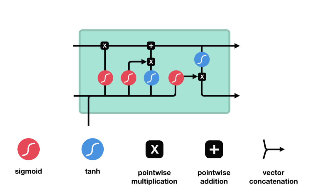
From the network structure diagram of LSTM, we can see that LSTM is actually a small model, which includes three sigmoid activation functions, two tanh activation functions, three multipliers and one addition.

Cellular state

Cell state is the core of LSTM. It is the top black line in the picture above. Below the black line are some doors. We will introduce them later. Cell status is updated based on the results of each gate. Let's introduce these gates, and you will understand the flow of cell state.

LSTM network can delete or add information to cell state through a structure called gate. Doors can selectively decide which messages to let through. The gate structure is a combination of a sigmoid layer and a point multiplication operation. Because the output of sigmoid layer is a value of 0-1, 0 means that it can not pass, and 1 means that it can pass. An LSTM contains three gates to control cell state. Let's introduce these doors one by one.

Oblivion gate

The first step of LSTM is to determine what information the cell status needs to discard. This part of the operation is handled by a sigmoid unit called forgetting gate. Let's take a look at the animation,

We can see that forgetting gate outputs a vector between 0-1 by looking at the information of $h {L-1} $and $X {t} $. The value of 0-1 in the vector indicates which information in cell state $C {T-1} $is retained or discarded. 0 means no reservation, 1 means all reservation.

Mathematical expression: $f {t} = \ Sigma \ left (w {f} \ cdot \ left [h {T-1}, X {t} \ right] + B {f} \ right)$

Input gate

The next step is to decide what new information to add to the cell state, which is done by opening the input door. Let's take a look at the animation,

We see that the information of $h {L-1} $and $X {t} $is put into a forgetting gate (sigmoid) and an input gate (tanh). Because the output of the forgetting gate is 0-1, if the output of the forgetting gate is 0, the result $C {I} $after the input gate will not be added to the current cell state, if it is 1, it will be all added to the cell state, so the function of the forgetting gate here is to selectively add the results of the input gate to the cell state.

The mathematical formula is: $C {t} = f {t} * C {T-1} + I {t} * \ \ tilde {C} {t}$

Output gate

After updating the cell state, we need to determine which state features of the output cell according to the sum of the input of $h {L-1} $and $X {t} $. Here, we need to pass the input through a sigmoid layer called the output gate to get the judging conditions, and then pass the cell state through the tanh layer to get a vector between - 1 and 1. The vector and the judging conditions obtained by the output gate are multiplied to get the final RNN unit output The animation diagram is as follows

def create_model():
    model = Sequential()
    model.add(LSTM(50, input_shape=(train_x.shape[1], train_x.shape[2])))
    model.add(Dense(1))
    model.compile(loss='mae', optimizer='adam')
    model.summary()
    return model

model = create_model()

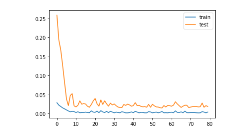
history = model.fit(train_x, train_y, epochs=80, batch_size=64, validation_data=(test_x, test_y), verbose=1, shuffle=False)

plt.plot(history.history['loss'], label='train')
plt.plot(history.history['val_loss'], label='test')
plt.legend()
plt.show()

train_x, train_y = create_dataset(train)
test_x, test_y = create_dataset(test)

forecast

predict = model.predict(test_x)
plt.plot(predict, label='predict')
plt.plot(test_y, label='ground true')
plt.legend()
plt.show()

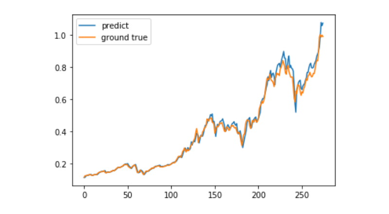
At present, it is very difficult to use machine learning to predict the long-term price trend of bitcoin. This paper can only be used as a learning case. The case will be online and in the Demo image of moment pool cloud later, and interested users can experience it directly.