matrix
The establishment of matrix
v=1:6
m=matrix(v,2,3) #Default load by column
m
[,1] [,2] [,3]
[1,] 1 3 5
[2,] 2 4 6
n=matrix(v,2,3,byrow=TRUE) #Load by line
n
[,1] [,2] [,3]
[1,] 1 2 3
[2,] 4 5 6
dim(m) #Matrix dimension
[1] 2 3
Matrix row and column naming
rownames(m)=c('male','female')#Named row
colnames(m)=c('low','middle','high')#Named column
dimnames(m)#View row and column names for the matrix
[[1]]
[1] "male" "female"
[[2]]
[1] "low" "middle" "high"
m#View matrix m
low middle high
male 1 3 5
female 2 4 6
Unit matrix
x=diag(3)
x
[,1] [,2] [,3]
[1,] 1 0 0
[2,] 0 1 0
[3,] 0 0 1
Diagonal matrix composed of diagonal elements of m
y=diag(m)
y
[1] 1 4
Taking elements in v as diagonal elements to form diagonal matrix
z=diag(v)
z
[,1] [,2] [,3] [,4] [,5] [,6]
[1,] 1 0 0 0 0 0
[2,] 0 2 0 0 0 0
[3,] 0 0 3 0 0 0
[4,] 0 0 0 4 0 0
[5,] 0 0 0 0 5 0
[6,] 0 0 0 0 0 6
Index of matrix and extraction of subset (element)
Rules: subscripts of the same vector
Generate 3 rows and 4 columns matrix
z=matrix(1:12,3,4)
z
[,1] [,2] [,3] [,4]
[1,] 1 4 7 10
[2,] 2 5 8 11
[3,] 3 6 9 12
Extract matrix elements in Row 2 and column 4
z[2,4]
[1] 11
Extract matrix elements of row 1, 2, column 2 and column 4
z[1:2,c(2,4)]
[,1] [,2]
[1,] 4 10
[2,] 5 11
Extract line 3
z[3,]
[1] 3 6 9 12
Extract column 2
z[,2]
[1] 4 5 6
Delete all matrix elements in row 1 and column 3
z[,-c(1,3)]
[,1] [,2]
[1,] 4 10
[2,] 5 11
[3,] 6 12
Replace the fourth column with the missing value
z[,4]=NA
z
[,1] [,2] [,3] [,4]
[1,] 1 4 7 NA
[2,] 2 5 8 NA
[3,] 3 6 9 NA
Replace missing value with 1
z[is.na(z)]=1
z
[,1] [,2] [,3] [,4]
[1,] 1 4 7 1
[2,] 2 5 8 1
[3,] 3 6 9 1
Matrix operation (function)
Algebraic operation
1. transpose t()
x = matrix(1:6, 2, 3)
x
[,1] [,2] [,3]
[1,] 1 3 5
[2,] 2 4 6
t(x)
[,1] [,2]
[1,] 1 2
[2,] 3 4
[3,] 5 6
Several matrix merges
y <- matrix(1:4, 2, 2)
y
[,1] [,2]
[1,] 1 3
[2,] 2 4
Merge by column with the same number of rows
cbind(x, y)
[,1] [,2] [,3] [,4] [,5]
[1,] 1 3 5 1 3
[2,] 2 4 6 2 4
Merge by row, requiring the same number of columns
z =matrix(-1:(-6), 2, 3, by=T)
z
[,1] [,2] [,3]
[1,] -1 -2 -3
[2,] -4 -5 -6
rbind(x, z)
[,1] [,2] [,3]
[1,] 1 3 5
[2,] 2 4 6
[3,] -1 -2 -3
[4,] -4 -5 -6
matrix multiplication
x
[,1] [,2] [,3]
[1,] 1 3 5
[2,] 2 4 6
z
[,1] [,2] [,3]
[1,] -1 -2 -3
[2,] -4 -5 -6
Multiplication of corresponding elements of two matrices of the same dimension
x*z
[,1] [,2] [,3]
[1,] -1 -6 -15
[2,] -8 -20 -36
Algebraic product of two matrices
x%*%t(z)
[,1] [,2]
[1,] -22 -49
[2,] -28 -64
Algebraic product of two matrices
tcrossprod(x, z)
[,1] [,2]
[1,] -22 -49
[2,] -28 -64
= t(x) %*% z
crossprod(x, z)
[,1] [,2] [,3]
[1,] -9 -12 -15
[2,] -19 -26 -33
[3,] -29 -40 -51
kronecker product
kronecker(x, z)
[,1] [,2] [,3] [,4] [,5] [,6] [,7] [,8] [,9]
[1,] -1 -2 -3 -3 -6 -9 -5 -10 -15
[2,] -4 -5 -6 -12 -15 -18 -20 -25 -30
[3,] -2 -4 -6 -4 -8 -12 -6 -12 -18
[4,] -8 -10 -12 -16 -20 -24 -24 -30 -36
Eigenvalue decomposition of matrix
y
[,1] [,2]
[1,] 1 3
[2,] 2 4
The return value is a list of values and vectors
ev=eigen(y)
ev
eigen() decomposition
$values
[1] 5.3722813 -0.3722813
$vectors
[,1] [,2]
[1,] -0.5657675 -0.9093767
[2,] -0.8245648 0.4159736
ev$values take out the eigenvalues (lambda1, lamda2 )
ev$vectors take out the corresponding eigenvectors (v1, v2 )
Because the code is printed out in random code, only TUT can be screenshot
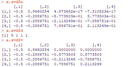
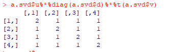
Singular value decomposition of matrix
A = UDV ', where U'U=V'v = I and D are diagonal matrices
Returns a list of d, u, v components
a
[,1] [,2] [,3] [,4]
[1,] 2 1 1 1
[2,] 1 2 1 1
[3,] 1 1 2 1
[4,] 1 1 1 2

Determinant of matrix a|
det(a)
[1] 5
Inverse of matrix ax=b
b=-1:2
x=solve(a,b)
b
[1] -1 0 1 2
x
[1] -1.4 -0.4 0.6 1.6
Verification
a%*%x
[,1]
[1,] -1.000000e+00
[2,] -2.220446e-16
[3,] 1.000000e+00
[4,] 2.000000e+00
inva, the inverse matrix of a
inva=solve(a)
inva
[,1] [,2] [,3] [,4]
[1,] 0.8 -0.2 -0.2 -0.2
[2,] -0.2 0.8 -0.2 -0.2
[3,] -0.2 -0.2 0.8 -0.2
[4,] -0.2 -0.2 -0.2 0.8
a%*%inva
[,1] [,2] [,3] [,4]
[1,] 1.000000e+00 0.000000e+00 -5.551115e-17 0
[2,] -8.326673e-17 1.000000e+00 -5.551115e-17 0
[3,] -1.110223e-16 1.665335e-16 1.000000e+00 0
[4,] -1.110223e-16 1.110223e-16 0.000000e+00 1
Straightening of matrix
as.vector(a)
[1] 2 1 1 1 1 2 1 1 1 1 2 1 1 1 1 2
Statistical operation
m=1:12
m=matrix(m,3,4)
m
[,1] [,2] [,3] [,4]
[1,] 1 4 7 10
[2,] 2 5 8 11
[3,] 3 6 9 12
apply(m, MARGIN=1, FUN=mean)
[1] 5.5 6.5 7.5
apply(m, MARGIN=2, FUN=median)
[1] 2 5 8 11
m.cen <- scale(m, center=T, scale=F)
m.cen
[,1] [,2] [,3] [,4]
[1,] -1 -1 -1 -1
[2,] 0 0 0 0
[3,] 1 1 1 1
attr(,"scaled:center")
[1] 2 5 8 11
apply(m.cen, MARGIN=2, FUN=mean)
[1] 0 0 0 0
m.stand <- scale(m, center=T, scale=T)
m.stand
[,1] [,2] [,3] [,4]
[1,] -1 -1 -1 -1
[2,] 0 0 0 0
[3,] 1 1 1 1
attr(,"scaled:center")
[1] 2 5 8 11
attr(,"scaled:scale")
[1] 1 1 1 1
apply(m.stand, MARGIN=2, FUN=mean)
[1] 0 0 0 0
apply(m.stand, MARGIN=2, FUN=sd)
[1] 1 1 1 1
row.med <- apply(m, MARGIN=1, FUN=median)
row.med
[1] 5.5 6.5 7.5
sweep(m, MARGIN=1, STATS=row.med, FUN="-")

