1, Foreword
When carrying out fundamental analysis on a listed company, we can usually analyze and interpret its financial data and evaluate its internal value through various channels such as research on listed companies. Our commonly used financial evaluation indicators may include:
1) Price earnings ratio (PE): market price per share / earnings per share; Also known as profit rate of return, it refers to the ratio of the market price of a common stock to earnings per share, which measures the performance of enterprise profits. Generally speaking, the higher the PE, the higher the public's evaluation of the stock.
2) Price to book ratio (PB): share price / net assets per share; Measure the ratio between the current stock price and the company's real net assets per share. Generally, the smaller the Pb, the higher the safety margin.
3) Market to sales ratio (PS): share price / earnings per share; It is suitable for measuring enterprises that have no profit or are really profitable, such as Internet companies and technology companies in the development period. In general, the more obvious PS is, the greater the current investment value of the company is.
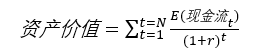
In addition, when measuring the value of listed companies and whether the stock value deviates, there is a more complex and rigorous model - discounted cash flow model (DCF), that is, discount all the cash flow of the enterprise's future operation and production to today, calculate its market price and compare it with the stock price to judge whether the price deviates. This paper will take Gree Electric Appliance (sz00651) Taking Python as an example, PE/PS index tracking and DCF model construction are carried out in detail.
2, Principle of DCF valuation model
The construction idea of discounted cash flow model (DCF) comes from bonds. It discounts all cash flows of the enterprise in the future duration to today to obtain the estimation of the internal value of the enterprise, which mainly includes three processes
2.1 model process
1) Free cash flow FCFF is calculated. Enterprise free cash flow is the discounted object in DCF model. It refers to the cash generated by the enterprise, remaining after meeting the reinvestment demand and without affecting the sustainable development of the company, which can be distributed by enterprise capital suppliers / various interest claimants (shareholders and creditors), That is, the free cash that can be created for distribution by shareholders and creditors based on the company's assets every year. The general calculation formula is:
Operating cash flow = net profit + financial expenses - investment income - income from disposal of fixed assets + amortization of fixed assets + provision for asset impairment + decrease in accounts receivable + decrease in inventory - increase in accounts payable + deferred income tax
Free cash flow = operating cash flow - capital expenditure - increase in goodwill investment
2) Calculate discount rate (WACC) After the free cash flow FCFF is calculated, the appropriate discount rate is selected to discount the cash flow according to the characteristics of the company's industry. Generally, the weighted average cost of capital rate (WACC) is selected, that is, the weighted average method of calculating the company's capital cost according to the weight of all kinds of capital in the total capital source.
Weighted average cost of capital (WACC) = proportion of equity to market value * expected rate of return of equity + proportion of creditor's rights to market value * (1 - tax rate) * cost of corporate debt
3) When discounting the cash flow, it is generally assumed that the future cash flow growth rate of the enterprise is g. according to the enterprise life cycle theory, the life cycle of the enterprise is divided into predictable stage and sustainable value stage. According to the life cycle theory, it is further divided into input stage, mature stage and recession stage, and different growth rates g1, g2 and g3 are given, The enterprise value is obtained by discounting the future cash flow to the current period.
two point two Mathematical principles
Since it is difficult to accurately predict the cash flow at every moment in the future, and the stock does not have a fixed life cycle, the general simplified models are constant growth model, two-stage model and three-stage model. Taking the constant growth model as an example, its free cash discount value can be expressed as:
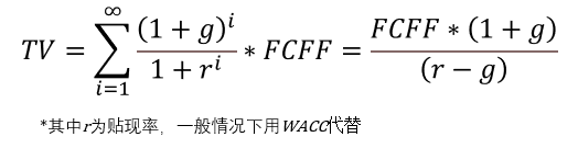
Where TV is the final value and g is the sustainable growth rate, that is, the assumed increase of future cash flow of the enterprise. In reality, the cash flow of each period continues to flow into the enterprise, but in order to simplify and facilitate the calculation, it is necessary to assume that the cash flow of each period flows in one time at a certain point in the period. Conventionally, it is assumed that the cash flow of each period is inflow during the period, which is equivalent to assuming that the cash flow of the current period is uniform inflow, so as to determine the number of discounted periods.
3, Process implementation based on Python
We select Gree Electric (sz00651) as an example to analyze each index in turn. Before analysis, we first need to obtain stock data and financial data of each dimension. Here we use financial quantitative data interface AKShare Open source financial data interface library for data acquisition.
import pandas as pd
import datetime
from matplotlib import pyplot as plt
import akshare as ak

 #Obtain all stock data of A shares and store them in stock_basic.csv
stock_zh=ak.stock_zh_a_spot()
stock_zh.to_csv("stock_basic.csv") 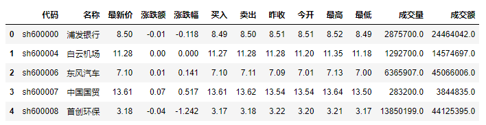
First, get the general picture of A-share market, get the real-time market data of A-share listed companies, then screen out the data of Gree Electric Appliance and observe its historical market data. Here, we re weight the data, keep the current price unchanged and increase or decrease the historical price, so as to make the stock price continuous. Based on this, we draw the "closing price" and "highest price" of Gree Electric appliance And "lowest price" data chart.
stock_zh.head()
stock_zh[stock_zh["name"]=="Gree Electric Appliance"]
stock_daily = ak.stock_zh_a_hist(symbol="000651", period="daily", start_date="20200101", end_date='20211104', adjust="qfq")
close_price=stock_daily[["date","closing quotation","highest","minimum"]]
close_price.set_index("date",inplace=True)

close_price.plot()
close_price.head()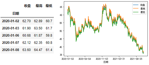
Next, we obtain the historical PE/PS data of Gree Electric Appliance, draw the data map and observe its historical trend more intuitively; It can be seen that the P / E ratio of Gree Electric Appliance remained stable at about 15 from November 2020 to may 2021, and decreased to 9 from September 2021 to November 2021, which is a good investment target.
#Get PE/PS and total market value
geli_df = ak.stock_a_lg_indicator(stock="000651")
geli_df.set_index("trade_date",inplace=True)
geli_pe_ps=geli_df.iloc[0:240,[0,3]]
geli_pe_ps.plot()
geli_df.head()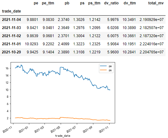
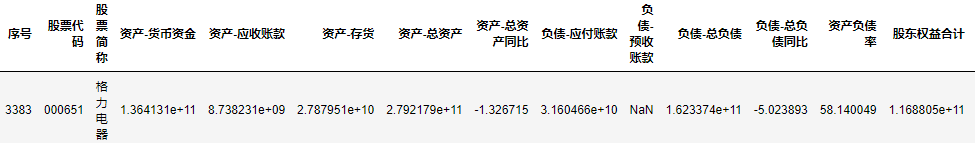
After completing PE and PS tracking, we build DCF valuation model to analyze the internal value of Gree Electric appliance. In order to avoid subtle differences in some data of quarterly and semi annual reports, we chose to obtain the financial summary and individual stock overview of Gree's annual report on December 31, 2020, so as to have a macro understanding of its operation in fiscal year 2020.
import numpy as np
import pandas as pd
import matplotlib as plt
import akshare as ak

#Get stock overview
dateset=["20200331", "20200630", "20200930", "20201231"]
stock_em_yjkb_df = ak.stock_em_yjkb(date="20201231")
geli_sheet=stock_em_yjkb_df[stock_em_yjkb_df['Stock code']=="000651"]
geli_sheet

#Get financial summary
stock_em_zcfz_df = ak.stock_em_zcfz(date="20201231")
geli_sheet2=stock_em_zcfz_df[stock_em_zcfz_df["Stock code"]=="000651" ]
geli_sheet2
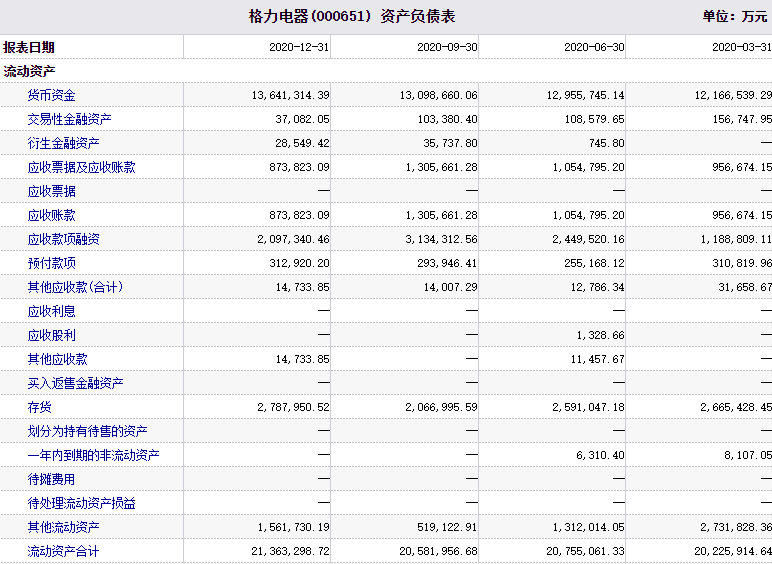
Next, we obtain three main tables, namely, balance sheet, income statement and cash flow statement. The data source is Sina Finance The report overview is shown in the figure below
#Obtain cash flow statement
stock_financial_report_sina_df = ak.stock_financial_report_sina(stock="000651", symbol="Cash flow statement")
geli_sheet1=stock_financial_report_sina_df[stock_financial_report_sina_df["Report date"]=="20201231"]
geli_sheet1

#Obtain income statement
stock_financial_report_sina_lrb = ak.stock_financial_report_sina(stock="000651", symbol="Income statement")
geli_sheet2=stock_financial_report_sina_lrb[stock_financial_report_sina_lrb["Report date"]=="20201231"]
geli_sheet2

#Obtain 20201231 balance sheet
stock_financial_report_sina_lrb = ak.stock_financial_report_sina(stock="000651", symbol="Balance sheet")
geli_sheet3=stock_financial_report_sina_lrb[stock_financial_report_sina_lrb["Report date"]=="20201231"]
geli_sheet3
#Obtain 20191231 balance sheet
stock_financial_report_sina_lrb = ak.stock_financial_report_sina(stock="000651", symbol="Balance sheet")
geli_sheet4=stock_financial_report_sina_lrb[stock_financial_report_sina_lrb["Report date"]=="20191231"]
geli_sheet4
Using the data of financial statements, we capture the data of necessary accounting subjects to calculate WACC, effective income tax rate, free cash flow FCF of the current year and other indicators; Wherein, the cost ratio of equity capital = risk-free rate of return + BETA coefficient × Market risk premium, and BETA coefficient is generally obtained by regression of data in previous years. Here, 9% is used as the cost rate of equity capital Ke.
###Operating cash flow = net profit + financial expenses - investment income - income from disposal of fixed assets + amortization of fixed assets + provision for asset impairment + decrease in accounts receivable + decrease in inventory - increase in accounts payable + deferred income tax
##Free cash flow = operating cash flow - capital expenditure - increase in goodwill investment
##Debt capital cost ratio = (interest expense + interest payable) / debt capital


#free cash flow
FCF=float(geli_sheet1["Net cash flow from operating activities"])-float(geli_sheet1["Depreciation of fixed assets, depletion of oil and gas assets and depreciation of productive materials"])-float(geli_sheet1["Amortization of intangible assets"])-float(geli_sheet1["Amortization of long-term deferred expenses"])-float(geli_sheet1["Losses from disposal of fixed assets, intangible assets and other long-term assets"])

#Effective income tax rate
E_Tax=1-(float(geli_sheet2["4, Total profit"])-float(geli_sheet2["Less: income tax expense"]))/float(geli_sheet2["4, Total profit"])

#Cost of capital and cost of equity
Kd=(float(geli_sheet2["Financial expenses"])+float(geli_sheet2["Exchange gains"]))/((float(geli_sheet3["Total liabilities"])+float(geli_sheet4["Total liabilities"]))/2)
#Kd=(float(geli_sheet2 ["financial expenses") + float(geli_sheet2 ["exchange gains")) / float(geli_sheet3 ["total liabilities"))
Ke=0.09 #The cost of equity is set at 9%

#Proportion of debt
Pd=float(geli_sheet3["Total liabilities"])/float(geli_sheet3["Liabilities and owner's equity(Or shareholders' equity)total"])

#Proportion of minority shareholders' equity
Me=float(geli_sheet3["Minority interests"])/float(geli_sheet3["Owner's equity(Or shareholders' equity)total"])

#WACC calculation
WACC=Kd*Pd*(1-E_Tax)+Ke*(1-Pd)
After obtaining WACC, we calculate the final value. Considering the business cycle of the enterprise, we choose the three-stage model for calculation (in fact, the three-stage model is not stable when evaluating Gree, because Gree has entered the mature stage or platform stage, its cash flow growth rate will not change significantly, and the three-stage model is more suitable for start-ups, etc.)
#Calculation of discount factor: taking three stages as an example
g1,g2,g3=0.3,0.15,0.02 #Three stage growth rate
t1,t2=np.arange(1,6), np.arange(1,6) #The growth period t1 is five years and the development period T2 is five years
EV_sum1, EV_sum2 = 0, 0
for _ in t1:
    EV1 = FCF * ((1+g1) ** _) #Forecast of future operation
    EV =  EV1 / ((1+WACC) ** _)
    EV_sum1 = EV + EV_sum1

for _ in t2:
    EV = EV1 * ((1+g2) ** _) / ((1+WACC) ** (_+t1[-1]))
    EV_sum2 = EV + EV_sum2

PDV = (EV1 * ((1+g2) ** t2[-1]) * (1+g3)) / ((WACC-g3)*((1+WACC)**(t1[-1]+t2[-1]))) + EV_sum1 + EV_sum2
PDV_adj =PDV* (1 - Me) #Adjustment of shareholders' equity
Finally, we calculate the total number of shares of Gree and estimate the intrinsic value of the stock. The results show that the current Gree stock price is close to the estimated price of DCF valuation model and does not deviate from its actual intrinsic value.
#Total number of shares
total_mv=geli_df.loc["2020-12-31","total_mv"]*10**4
close=close_price.loc["2020-12-31","closing quotation"]
Shares=total_mv/close

Value = PDV_adj / Shares
print('Value attributable to shareholders of listed companies:',PDV_adj, '\n', 'Intrinsic value:', Value)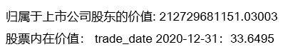
In the process of further application, we should make a more prudent judgment on the discount rate and sustainable growth rate of the model, because the degree of security or risk implied when we adopt various valuation States is also very different under different circumstances. Therefore, we should conduct a more in-depth sensitivity analysis and then choose a safer strategic investment.
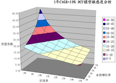 DCF model sensitivity analysis (Figure: Barrons blog)
reference
[1] Guo Yongqing. Financial statement analysis and stock valuation. [D]: China Machine Press
[2] Understanding the core logic of DCF model
[3] [programming] DCF free cash flow discount model -- Implementation Based on python