Pytorch Note53 TensorBoard Visualization
A summary of all notes: Pytorch Note Happy Planet
TensorBoard is a visualization tool for Tensorflow that visualizes the running state of Tensorflow programs through the log files that are output during the running of the Tensorflow program.TensorBoards and TensorFlow programs run in different processes. TensorBoards automatically read the latest TensorFlow log files and present the latest status of the current TensorFlow program.
In addition to Tensorflow, you can also visualize our Pytorch
Install TensorBoard
It's easy to install TensorBoard first. We use cmd to open our command line, and then enter the following command
pip install tensorboard
Then install it successfully
We can test whether the installation was successful, and we can enter the following command in our cmd command
tensorboard --logdir=D:\
If there is a result, we have successfully installed
Use of TensorBoard
Once the installation is complete, let's demonstrate the visualization of TensorBoard with an example
# imports
import matplotlib.pyplot as plt
import numpy as np

import torch
import torchvision
import torchvision.transforms as transforms

import torch.nn as nn
import torch.nn.functional as F
import torch.optim as optim

# transforms
transform = transforms.Compose(
    [transforms.ToTensor(),
    transforms.Normalize((0.5,), (0.5,))])

# datasets
trainset = torchvision.datasets.FashionMNIST('./data',
    download=True,
    train=True,
    transform=transform)
testset = torchvision.datasets.FashionMNIST('./data',
    download=True,
    train=False,
    transform=transform)

# dataloaders
trainloader = torch.utils.data.DataLoader(trainset, batch_size=4,
                                        shuffle=True, num_workers=2)

testloader = torch.utils.data.DataLoader(testset, batch_size=4,
                                        shuffle=False, num_workers=2)

# constant for classes
classes = ('T-shirt/top', 'Trouser', 'Pullover', 'Dress', 'Coat',
        'Sandal', 'Shirt', 'Sneaker', 'Bag', 'Ankle Boot')

# helper function to show an image
# (used in the `plot_classes_preds` function below)
def matplotlib_imshow(img, one_channel=False):
    if one_channel:
        img = img.mean(dim=0)
    img = img / 2 + 0.5     # unnormalize
    npimg = img.numpy()
    if one_channel:
        plt.imshow(npimg, cmap="Greys")
    else:
        plt.imshow(np.transpose(npimg, (1, 2, 0)))
In this tutorial, we will define a similar model architecture that addresses the fact that the image is now a channel, not three channels, and the image is 28x28 instead of 32x32 with only a few modifications:
class Net(nn.Module):
    def __init__(self):
        super(Net, self).__init__()
        self.conv1 = nn.Conv2d(1, 6, 5)
        self.pool = nn.MaxPool2d(2, 2)
        self.conv2 = nn.Conv2d(6, 16, 5)
        self.fc1 = nn.Linear(16 * 4 * 4, 120)
        self.fc2 = nn.Linear(120, 84)
        self.fc3 = nn.Linear(84, 10)

    def forward(self, x):
        x = self.pool(F.relu(self.conv1(x)))
        x = self.pool(F.relu(self.conv2(x)))
        x = x.view(-1, 16 * 4 * 4)
        x = F.relu(self.fc1(x))
        x = F.relu(self.fc2(x))
        x = self.fc3(x)
        return x

net = Net()
We'll define the same optimizer and criterion before:
criterion = nn.CrossEntropyLoss()
optimizer = optim.SGD(net.parameters(), lr=0.001, momentum=0.9)
1. TensorBoard settings
Now we'll set up TensorBoard, import tensorboard from torch.utils, and define SummaryWriter, which is the key object for writing information to TensorBoard.
from torch.utils.tensorboard import SummaryWriter

# default `log_dir` is "runs" - we'll be more specific here
writer = SummaryWriter('runs/fashion_mnist_experiment_1')
Note that only this line creates a runs/fashion_mnist_experiment_1 folder.
2. Write to TensorBoard
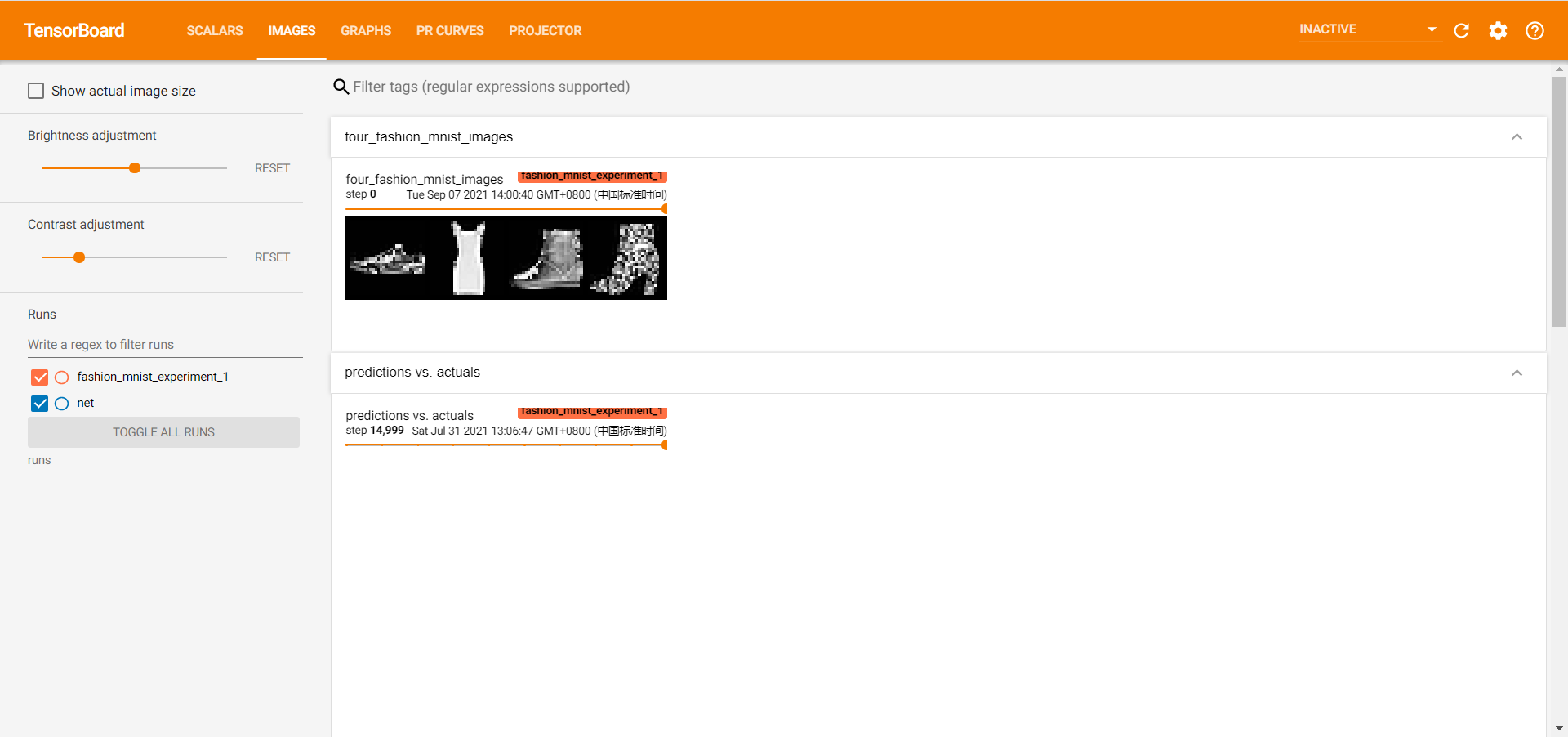
Now, use make_The grid writes the image to TensorBoard, specifically the grid.
# get some random training images
dataiter = iter(trainloader)
images, labels = dataiter.next()

# create grid of images
img_grid = torchvision.utils.make_grid(images)

# show images
matplotlib_imshow(img_grid, one_channel=True)

# write to tensorboard
writer.add_image('four_fashion_mnist_images', img_grid)

images.shape
torch.Size([4, 1, 28, 28])
Start TensorBoard
Run the following command to start TensorBoard
load_ext tensorboard
tensorboard --logdir=runs
Running the above command starts a service with the parent's port defaulting to 6006.Open localhost:6006 from your browser.You can change the port on which the service is started by using the - port parameter.
Open TensorBoard as follows:
3. Check the model using TensorBoard
One of the advantages of TensorBoard is its ability to visualize complex model structures.Let's visualize the model we built.
writer.add_graph(net, images)
writer.close()
Continue and double-click Net to expand it to see a detailed view of the operations that make up the model.
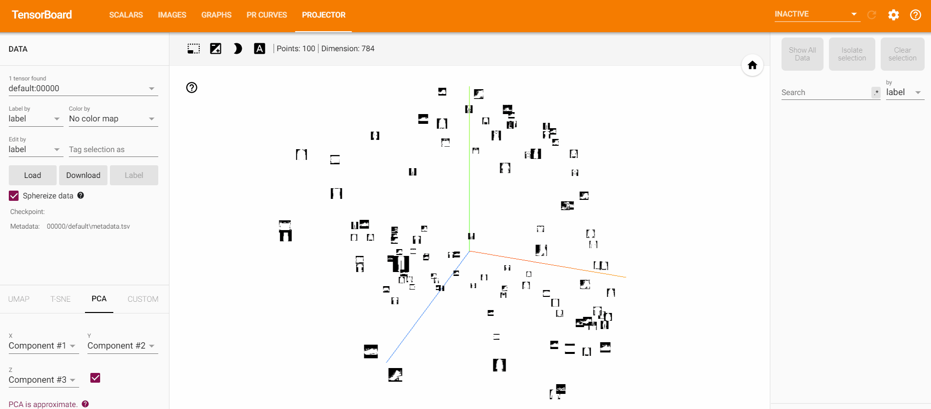
TensorBoard has a very convenient function to visualize high-dimensional data, such as image data, in low-dimensional space.Next we'll cover that.
[External chain picture transfer failed, source station may have anti-theft chain mechanism, it is recommended to save the picture and upload it directly (img-S8hmk7Nm-163085998) (C:Users137AppDataRoamingTyporatypora-user-imagesimage-2021450.png)]
4. Add "Projector" to TensorBoard
We can add_embedding method visualizes low-dimensional representation of high-dimensional data
import tensorboard as tb
import tensorflow as tf
tf.io.gfile = tb.compat.tensorflow_stub.io.gfile
# helper function
def select_n_random(data, labels, n=100):
    '''
    Selects n random datapoints and their corresponding labels from a dataset
    '''
    assert len(data) == len(labels)

    perm = torch.randperm(len(data))
    return data[perm][:n], labels[perm][:n]

# select random images and their target indices
images, labels = select_n_random(trainset.data, trainset.targets)

# get the class labels for each image
class_labels = [classes[lab] for lab in labels]

# log embeddings
features = images.view(-1, 28 * 28)
writer.add_embedding(features,
                    metadata=class_labels,
                    label_img=images.unsqueeze(1))
writer.close()
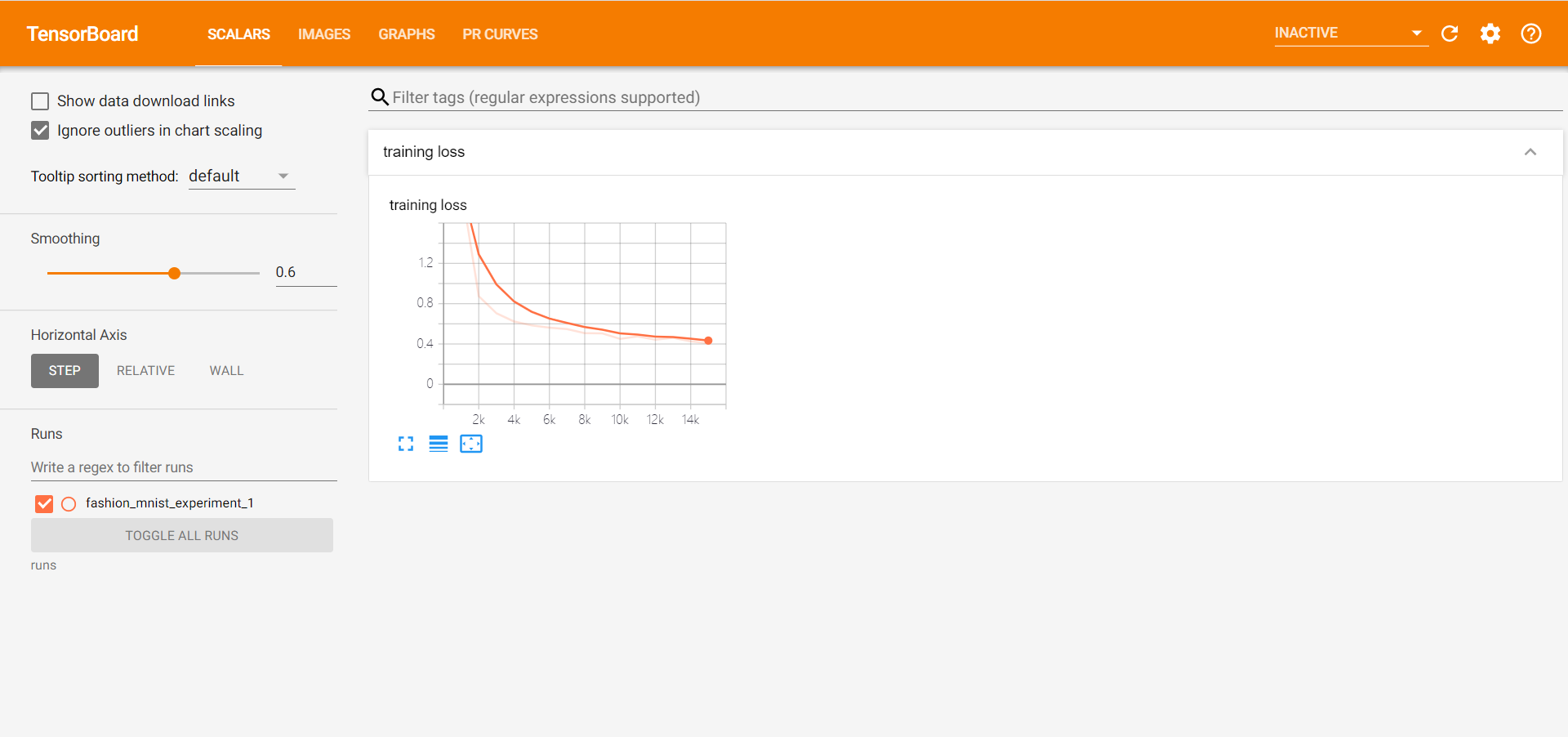
5. Tracking model training using TensorBoard
In the previous example, we only printed the loss of operation of the model every 2000 iterations.Now we will record the run loss in TensorBoard and pass plot_Classes_The preds function looks at the predictions made by the model.
# helper functions

def images_to_probs(net, images):
    '''
    Generates predictions and corresponding probabilities from a trained
    network and a list of images
    '''
    output = net(images)
    # convert output probabilities to predicted class
    _, preds_tensor = torch.max(output, 1)
    preds = np.squeeze(preds_tensor.numpy())
    return preds, [F.softmax(el, dim=0)[i].item() for i, el in zip(preds, output)]

def plot_classes_preds(net, images, labels):
    '''
    Generates matplotlib Figure using a trained network, along with images
    and labels from a batch, that shows the network's top prediction along
    with its probability, alongside the actual label, coloring this
    information based on whether the prediction was correct or not.
    Uses the "images_to_probs" function.
    '''
    preds, probs = images_to_probs(net, images)
    # plot the images in the batch, along with predicted and true labels
    fig = plt.figure(figsize=(12, 48))
    for idx in np.arange(4):
        ax = fig.add_subplot(1, 4, idx+1, xticks=[], yticks=[])
        matplotlib_imshow(images[idx], one_channel=True)
        ax.set_title("{0}, {1:.1f}%\n(label: {2})".format(
            classes[preds[idx]],
            probs[idx] * 100.0,
            classes[labels[idx]]),
                    color=("green" if preds[idx]==labels[idx].item() else "red"))
    return fig
running_loss = 0.0
for epoch in range(1):  # loop over the dataset multiple times

    for i, data in enumerate(trainloader, 0):

        # get the inputs; data is a list of [inputs, labels]
        inputs, labels = data

        # zero the parameter gradients
        optimizer.zero_grad()

        # forward + backward + optimize
        outputs = net(inputs)
        loss = criterion(outputs, labels)
        loss.backward()
        optimizer.step()

        running_loss += loss.item()
        if i % 1000 == 999:    # every 1000 mini-batches...

            # ...log the running loss
            writer.add_scalar('training loss',
                            running_loss / 1000,
                            epoch * len(trainloader) + i)

            # ...log a Matplotlib Figure showing the model's predictions on a
            # random mini-batch
            writer.add_figure('predictions vs. actuals',
                            plot_classes_preds(net, inputs, labels),
                            global_step=epoch * len(trainloader) + i)
            running_loss = 0.0
print('Finished Training')
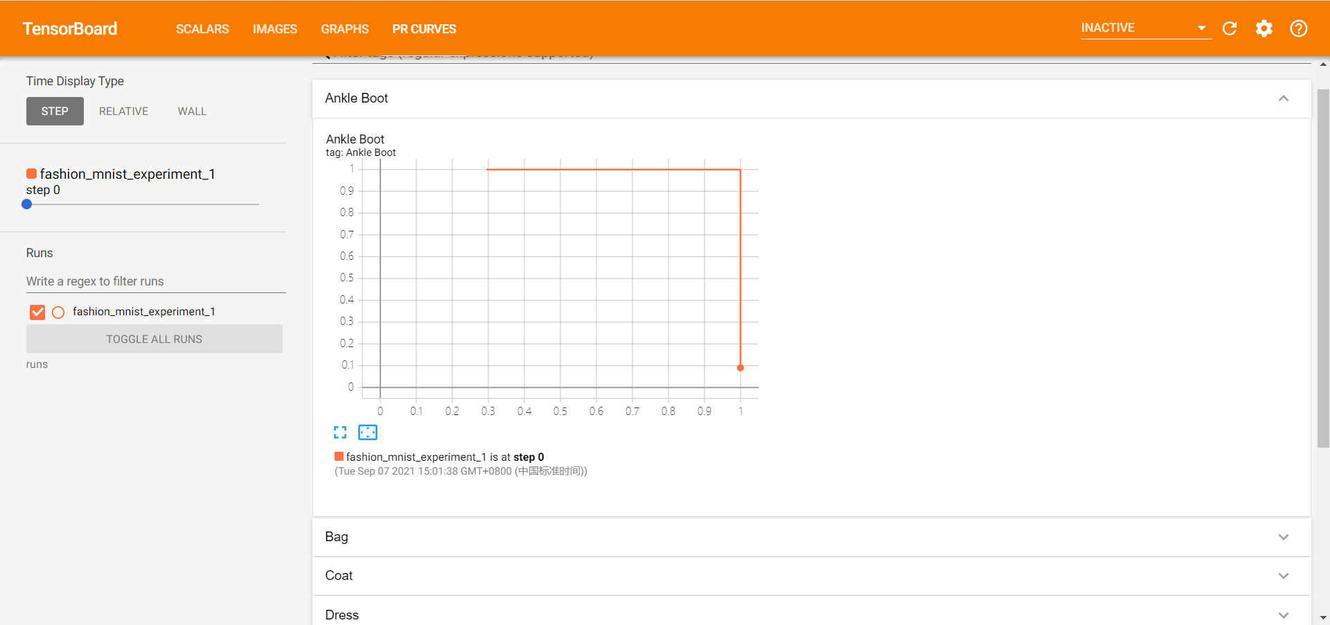
6. Use TensorBoard to evaluate trained models
We can get the probability of each class and our final PR curve
# 1\. gets the probability predictions in a test_size x num_classes Tensor
# 2\. gets the preds in a test_size Tensor
# takes ~10 seconds to run
class_probs = []
class_preds = []
with torch.no_grad():
    for data in testloader:
        images, labels = data
        output = net(images)
        class_probs_batch = [F.softmax(el, dim=0) for el in output]
        _, class_preds_batch = torch.max(output, 1)

        class_probs.append(class_probs_batch)
        class_preds.append(class_preds_batch)

test_probs = torch.cat([torch.stack(batch) for batch in class_probs])
test_preds = torch.cat(class_preds)

# helper function
def add_pr_curve_tensorboard(class_index, test_probs, test_preds, global_step=0):
    '''
    Takes in a "class_index" from 0 to 9 and plots the corresponding
    precision-recall curve
    '''
    tensorboard_preds = test_preds == class_index
    tensorboard_probs = test_probs[:, class_index]

    writer.add_pr_curve(classes[class_index],
                        tensorboard_preds,
                        tensorboard_probs,
                        global_step=global_step)
    writer.close()

# plot all the pr curves
for i in range(len(classes)):
    add_pr_curve_tensorboard(i, test_probs, test_preds)
Common problems
Here's a list of some of the problems I have with TensorBoard so that you don't have to make any detours
1. Kill the process
We can kill all TensorBoard processes with the following commands
taskkill /im tensorboard.exe /f
Success: Process terminated "tensorboard.exe",his PID 6948.
Success: Process terminated "tensorboard.exe",his PID It is 25888.
Or it might appear
error: No process found "tensorboard.exe".
Indicates that there is no process for tensorboard.
If not, we can also switch to another port.
2. Port occupied
As mentioned earlier, our default port is 6006. When we have more than one program, we may need to change the port, so we can modify our command to start TensorBoard, for example, by changing our port to 6008
tensorboard --logdir=runs --port=6008
That way, we can open port 6008 successfully.
3. Restart TensorBoard
reload_ext tensorboard
Example
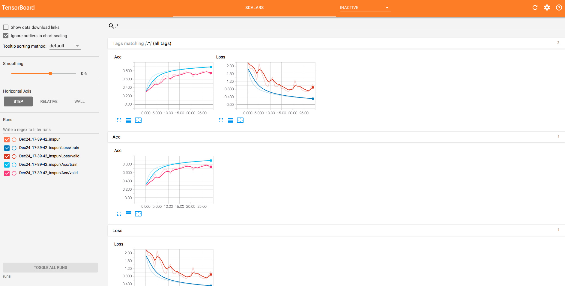
In fact, for us, sometimes we use TensorBoard s to visualize our losses and accuracy rather than so many results, so for us, it's very simple. Here's an example
writer = SummaryWriter()

def get_acc(output, label):
    total = output.shape[0]
    _, pred_label = output.max(1)
    num_correct = (pred_label == label).sum().data[0]
    return num_correct / total

if torch.cuda.is_available():
    net = net.cuda()
prev_time = datetime.now()
for epoch in range(30):
    train_loss = 0
    train_acc = 0
    net = net.train()
    for im, label in train_data:
        if torch.cuda.is_available():
            im = Variable(im.cuda())  # (bs, 3, h, w)
            label = Variable(label.cuda())  # (bs, h, w)
        else:
            im = Variable(im)
            label = Variable(label)
        # forward
        output = net(im)
        loss = criterion(output, label)
        # backward
        optimizer.zero_grad()
        loss.backward()
        optimizer.step()

        train_loss += loss.data[0]
        train_acc += get_acc(output, label)
    cur_time = datetime.now()
    h, remainder = divmod((cur_time - prev_time).seconds, 3600)
    m, s = divmod(remainder, 60)
    time_str = "Time %02d:%02d:%02d" % (h, m, s)
    valid_loss = 0
    valid_acc = 0
    net = net.eval()
    for im, label in valid_data:
        if torch.cuda.is_available():
            im = Variable(im.cuda(), volatile=True)
            label = Variable(label.cuda(), volatile=True)
        else:
            im = Variable(im, volatile=True)
            label = Variable(label, volatile=True)
        output = net(im)
        loss = criterion(output, label)
        valid_loss += loss.data[0]
        valid_acc += get_acc(output, label)
    epoch_str = (
                "Epoch %d. Train Loss: %f, Train Acc: %f, Valid Loss: %f, Valid Acc: %f, "
                % (epoch, train_loss / len(train_data),
                   train_acc / len(train_data), valid_loss / len(valid_data),
                   valid_acc / len(valid_data)))
    prev_time = cur_time
    # ============================Use tensorboard ===============
    writer.add_scalars('Loss', {'train': train_loss / len(train_data),
                                'valid': valid_loss / len(valid_data)}, epoch)
    writer.add_scalars('Acc', {'train': train_acc / len(train_data),
                               'valid': valid_acc / len(valid_data)}, epoch)
    # =========================================================
    print(epoch_str + time_str)