How to use skip-gram structure to implement Word2Vec algorithm in PyTorch? Embedding words used in natural language processing into concepts. Word embedding is very useful for machine translation.

Word Embedding

When dealing with words in text, thousands of word categories need to be analyzed; each word in the vocabulary corresponds to a category. It is very inefficient to encode these words by monotherm because most of the values in the monotherm vector will be zero. If the single heat input vector is multiplied by a matrix with the first hidden layer, a hidden output vector with multiple values of 0 will be generated. To solve this problem and improve the efficiency of the network, the embedded function will be used. Embedding is actually a fully connected layer, just like the level you've seen before. The hierarchy is called the embedding layer and the weight is called the embedding weight. The step of multiplying with the embedding layer is skipped and the hidden layer value is obtained directly from the weight matrix. This is because the result of multiplying the uniheat vector with the matrix is the matrix row corresponding to the index of the "open" input unit.

Word2Vec

Word2Vec algorithm finds the vectors representing words to get a more efficient representation. These vectors also contain semantic information about words. Words that appear in similar contexts will have vectors that are close to each other, such as "coffee", "tea" and "water". The vectors of different words are farther away from each other, and the distance in vector space can represent the relationship between words. Skp-gram structure and negative sampling will be used, because skip-gram is better than CBOW and the training speed of negative sampling is faster. For skip-gram structure, a word is passed in and an attempt is made to predict its contextual words in the text. In this way, we can train the network to learn the representation of words in similar contexts.

Loading data

Load the data and place it in the data directory.

# read in the extracted text file      
with open('data/text8/text8') as f:
    text = f.read()

# print out the first 100 characters
print(text[:100])

Pretreatment

Pre-processing text makes the training process more convenient. The preprocess function in the utils.py file performs the following operations:

• All punctuation points are converted to tags, so "." becomes <PERIOD>. Although this data set has no punctuation, this step is useful for other NLP problems.
• Delete words that appear no more than five times in the data set. This can significantly reduce the problems caused by data noise and improve the quality of vector representation.
• Returns a list of words in the text.

utils.py 

import re
from collections import Counter

def preprocess(text):

    # Replace punctuation with tokens so we can use them in our model
    text = text.lower()
    text = text.replace('.', ' <PERIOD> ')
    text = text.replace(',', ' <COMMA> ')
    text = text.replace('"', ' <QUOTATION_MARK> ')
    text = text.replace(';', ' <SEMICOLON> ')
    text = text.replace('!', ' <EXCLAMATION_MARK> ')
    text = text.replace('?', ' <QUESTION_MARK> ')
    text = text.replace('(', ' <LEFT_PAREN> ')
    text = text.replace(')', ' <RIGHT_PAREN> ')
    text = text.replace('--', ' <HYPHENS> ')
    text = text.replace('?', ' <QUESTION_MARK> ')
    # text = text.replace('\n', ' <NEW_LINE> ')
    text = text.replace(':', ' <COLON> ')
    words = text.split()
    
    # Remove all words with  5 or fewer occurences
    word_counts = Counter(words)
    trimmed_words = [word for word in words if word_counts[word] > 5]

    return trimmed_words


def create_lookup_tables(words):
    """
    Create lookup tables for vocabulary
    :param words: Input list of words
    :return: Two dictionaries, vocab_to_int, int_to_vocab
    """
    word_counts = Counter(words)
    # sorting the words from most to least frequent in text occurrence
    sorted_vocab = sorted(word_counts, key=word_counts.get, reverse=True)
    # create int_to_vocab dictionaries
    int_to_vocab = {ii: word for ii, word in enumerate(sorted_vocab)}
    vocab_to_int = {word: ii for ii, word in int_to_vocab.items()}

    return vocab_to_int, int_to_vocab

import utils

# get list of words
words = utils.preprocess(text)
print(words[:30])

# print some stats about this word data
print("Total words in text: {}".format(len(words)))
print("Unique words: {}".format(len(set(words)))) # `set` removes any duplicate words

Dictionaries

Two dictionaries will be created, one converting words to integers and the other converting integers to words. Also, use a function in the utils.py file to complete this step. The input parameter of create_lookup_tables is a list of text words and returns two dictionaries.

• Distributing integers in descending order of frequency, the most common word "the" corresponds to an integer of 0, the second common word is 1, and so on.

After the dictionary is created, the words are converted to integers and stored in the int_words list.

vocab_to_int, int_to_vocab = utils.create_lookup_tables(words)
int_words = [vocab_to_int[word] for word in words]

print(int_words[:30])

Secondary sampling

Frequent words such as "the", "of" and "for" do not provide much contextual information for nearby words. If some common words are discarded, some noise points in the data can be eliminated, and the training speed and the quality of the representation can be improved. Mikolov calls this process secondary sampling. For each word in the training set, the word will be discarded according to a certain probability. The formula is as follows:

                                                                            

Among them, t is the threshold parameter, and () is the frequency of words in the total data set.

Words in int_words were sampled twice. That is to access int_words and discard each word according to the probability shown above. Note that _ (_) denotes the probability of discarding a word. The secondary sampling data is assigned to train_words.

from collections import Counter
import random
import numpy as np

threshold = 1e-5
word_counts = Counter(int_words)
#print(list(word_counts.items())[0])  # dictionary of int_words, how many times they appear

total_count = len(int_words)
freqs = {word: count/total_count for word, count in word_counts.items()}
p_drop = {word: 1 - np.sqrt(threshold/freqs[word]) for word in word_counts}
# discard some frequent words, according to the subsampling equation
# create a new list of words for training
train_words = [word for word in int_words if random.random() < (1 - p_drop[word])]

print(train_words[:30])
print(len(Counter(train_words)))

Create batches

Once the data is ready, it needs to be batched before it can be transferred to the network. When using skip-gram structure, for each word in the text, you need to define a context window (size is_) and then get all the words in the window.

def get_target(words, idx, window_size=5):
    ''' Get a list of words in a window around an index. '''
    
    R = np.random.randint(1, window_size+1)
    start = idx - R if (idx - R) > 0 else 0
    stop = idx + R
    target_words = words[start:idx] + words[idx+1:stop+1]
    
    return list(target_words)

# test your code!

# run this cell multiple times to check for random window selection
int_text = [i for i in range(10)]
print('Input: ', int_text)
idx=5 # word index of interest

target = get_target(int_text, idx=idx, window_size=5)
print('Target: ', target)  # you should get some indices around the idx

Generate batch data

The following generator function will use the above get_target function to return multiple batches of input and target data. It retrieves the word batch_size from the list of words. For each batch of data, it retrieves the target context words in the window.

def get_batches(words, batch_size, window_size=5):
    ''' Create a generator of word batches as a tuple (inputs, targets) '''
    
    n_batches = len(words)//batch_size
    
    # only full batches
    words = words[:n_batches*batch_size]
    
    for idx in range(0, len(words), batch_size):
        x, y = [], []
        batch = words[idx:idx+batch_size]
        for ii in range(len(batch)):
            batch_x = batch[ii]
            batch_y = get_target(batch, ii, window_size)
            y.extend(batch_y)
            x.extend([batch_x]*len(batch_y))
        yield x, y
    

int_text = [i for i in range(20)]
x,y = next(get_batches(int_text, batch_size=4, window_size=5))

print('x\n', x)
print('y\n', y)

Verification

Next, create a function that will observe the model in the process of model learning. Some common and unusual words will be selected. Then use the similarity cosine to output the closest word. We use the embedded table to represent the validated words as vectors, and then calculate the similarity between the vectors of each word in the embedded table. After calculating the similarity, we will output validation words and words with similar semantics in the embedded table. This allows us to check whether the embedded table combines words with similar semantics.

def cosine_similarity(embedding, valid_size=16, valid_window=100, device='cpu'):
    """ Returns the cosine similarity of validation words with words in the embedding matrix.
        Here, embedding should be a PyTorch embedding module.
    """
    
    # Here we're calculating the cosine similarity between some random words and 
    # our embedding vectors. With the similarities, we can look at what words are
    # close to our random words.
    
    # sim = (a . b) / |a||b|
    
    embed_vectors = embedding.weight
    
    # magnitude of embedding vectors, |b|
    magnitudes = embed_vectors.pow(2).sum(dim=1).sqrt().unsqueeze(0)
    
    # pick N words from our ranges (0,window) and (1000,1000+window). lower id implies more frequent 
    valid_examples = np.array(random.sample(range(valid_window), valid_size//2))
    valid_examples = np.append(valid_examples,
                               random.sample(range(1000,1000+valid_window), valid_size//2))
    valid_examples = torch.LongTensor(valid_examples).to(device)
    
    valid_vectors = embedding(valid_examples)
    similarities = torch.mm(valid_vectors, embed_vectors.t())/magnitudes
        
    return valid_examples, similarities

Negative sampling

For each sample provided to the network, we use the output of the software max level to train the sample. This means that for each input, we will make minor adjustments to millions of weights, although there is only one real sample. This leads to the network training efficiency is very low. We can approximate the loss at the softmax level by updating only a small portion of the weight at a time. We will update the weights of the correct samples, but only the weights of a few incorrect samples. This process is called negative sampling.

We need to make two corrections: first, because we don't need to get the soft max output of all words, we only care about one output word at a time. Just like using an embedded table to map input words to the hidden layer, we can now use another embedded table to map the hidden layer to output words. Now we will have two embedding layers, one is the input word embedding layer, the other is the output word embedding layer. Secondly, we will modify the loss function because we only care about real samples and a small number of noise samples.

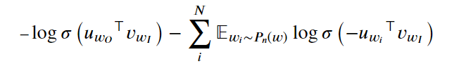
This loss function is somewhat complicated. It is the embedding vector of the target word "output" (the transposed vector, that is, the meaning of the symbol). It is the embedding vector of the word "input". The meaning of the first item is

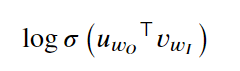
The log-sigmoid function is run on the inner product of the output word vector and the input word vector. For the second item, let's look at it first.

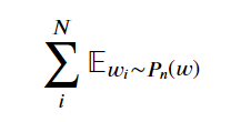
It means the sum of words extracted from the distribution of noise points. Noise distribution refers to a vocabulary that is not in the context of the input word. In fact, we can randomly extract words from the vocabulary to obtain these noisy words. The _ is an arbitrary probability distribution, so we can decide how to set the weight of the extracted words. It can be a uniform distribution, that is, the probability of extracting all words is the same. It can also be sampled according to the frequency at which each word appears in the text corpus. According to the author's practice, the best distribution is 3/4.

Finally, in the following sections

We will run the log-sigmoid function for the negative result of the inner product of the noise vector and the input vector.

import torch
from torch import nn
import torch.optim as optim

class SkipGramNeg(nn.Module):
    def __init__(self, n_vocab, n_embed, noise_dist=None):
        super().__init__()
        
        self.n_vocab = n_vocab
        self.n_embed = n_embed
        self.noise_dist = noise_dist
        
        # define embedding layers for input and output words
        self.in_embed = nn.Embedding(n_vocab,n_embed)
        self.out_embed = nn.Embedding(n_vocab,n_embed)
        
        # Initialize both embedding tables with uniform distribution
        
    def forward_input(self, input_words):
        # return input vector embeddings
        input_vectors = self.in_embed(input_words)
        return input_vectors
    
    def forward_output(self, output_words):
        # return output vector embeddings
        output_vectors = self.out_embed(output_words)
        return output_vectors
    
    def forward_noise(self, batch_size, n_samples):
        """ Generate noise vectors with shape (batch_size, n_samples, n_embed)"""
        if self.noise_dist is None:
            # Sample words uniformly
            noise_dist = torch.ones(self.n_vocab)
        else:
            noise_dist = self.noise_dist
            
        # Sample words from our noise distribution
        noise_words = torch.multinomial(noise_dist,
                                        batch_size * n_samples,
                                        replacement=True)
        
        device = "cuda" if model.out_embed.weight.is_cuda else "cpu"
        noise_words = noise_words.to(device)
        
        ## TODO: get the noise embeddings
        # reshape the embeddings so that they have dims (batch_size, n_samples, n_embed)
        
        noise_vectors = self.out_embed(noise_words).view(batch_size,n_sample,self.n_embed)
        
        return noise_vectors

class NegativeSamplingLoss(nn.Module):
    def __init__(self):
        super().__init__()

    def forward(self, input_vectors, output_vectors, noise_vectors):
        
        batch_size, embed_size = input_vectors.shape
        
        # Input vectors should be a batch of column vectors
        input_vectors = input_vectors.view(batch_size, embed_size, 1)
        
        # Output vectors should be a batch of row vectors
        output_vectors = output_vectors.view(batch_size, 1, embed_size)
        
        # bmm = batch matrix multiplication
        # correct log-sigmoid loss
        out_loss = torch.bmm(output_vectors, input_vectors).sigmoid().log()
        out_loss = out_loss.squeeze()
        
        # incorrect log-sigmoid loss
        noise_loss = torch.bmm(noise_vectors.neg(), input_vectors).sigmoid().log()
        noise_loss = noise_loss.squeeze().sum(1)  # sum the losses over the sample of noise vectors

        # negate and sum correct and noisy log-sigmoid losses
        # return average batch loss
        return -(out_loss + noise_loss).mean()

train

The following is the training cycle. If there is a GPU device, it is recommended to train the model on the GPU device.

device = 'cuda' if torch.cuda.is_available() else 'cpu'

# Get our noise distribution
# Using word frequencies calculated earlier in the notebook
word_freqs = np.array(sorted(freqs.values(), reverse=True))
unigram_dist = word_freqs/word_freqs.sum()
noise_dist = torch.from_numpy(unigram_dist**(0.75)/np.sum(unigram_dist**(0.75)))

# instantiating the model
embedding_dim = 300
model = SkipGramNeg(len(vocab_to_int), embedding_dim, noise_dist=noise_dist).to(device)

# using the loss that we defined
criterion = NegativeSamplingLoss() 
optimizer = optim.Adam(model.parameters(), lr=0.003)

print_every = 1500
steps = 0
epochs = 5

# train for some number of epochs
for e in range(epochs):
    
    # get our input, target batches
    for input_words, target_words in get_batches(train_words, 512):
        steps += 1
        inputs, targets = torch.LongTensor(input_words), torch.LongTensor(target_words)
        inputs, targets = inputs.to(device), targets.to(device)
        
        # input, outpt, and noise vectors
        input_vectors = model.forward_input(inputs)
        output_vectors = model.forward_output(targets)
        noise_vectors = model.forward_noise(inputs.shape[0], 5)

        # negative sampling loss
        loss = criterion(input_vectors, output_vectors, noise_vectors)

        optimizer.zero_grad()
        loss.backward()
        optimizer.step()

        # loss stats
        if steps % print_every == 0:
            print("Epoch: {}/{}".format(e+1, epochs))
            print("Loss: ", loss.item()) # avg batch loss at this point in training
            valid_examples, valid_similarities = cosine_similarity(model.in_embed, device=device)
            _, closest_idxs = valid_similarities.topk(6)

            valid_examples, closest_idxs = valid_examples.to('cpu'), closest_idxs.to('cpu')
            for ii, valid_idx in enumerate(valid_examples):
                closest_words = [int_to_vocab[idx.item()] for idx in closest_idxs[ii]][1:]
                print(int_to_vocab[valid_idx.item()] + " | " + ', '.join(closest_words))
            print("...\n")

Visual Word Vector

Next, we will use T-SNE to visualize high-dimensional word vector clustering. T-SNE can project these vectors into two-dimensional space while retaining local structure.

%matplotlib inline
%config InlineBackend.figure_format = 'retina'

import matplotlib.pyplot as plt
from sklearn.manifold import TSNE

# getting embeddings from the embedding layer of our model, by name
embeddings = model.in_embed.weight.to('cpu').data.numpy()

viz_words = 380
tsne = TSNE()
embed_tsne = tsne.fit_transform(embeddings[:viz_words, :])

fig, ax = plt.subplots(figsize=(16, 16))
for idx in range(viz_words):
    plt.scatter(*embed_tsne[idx, :], color='steelblue')
    plt.annotate(int_to_vocab[idx], (embed_tsne[idx, 0], embed_tsne[idx, 1]), alpha=0.7)