1. sklearn Profile
Scikit-learning is a common third-party module in machine learning. It encapsulates common machine learning methods, including Regression, Dimensional Reduction, Classification and Clustering.
Commonly used regression: linear, decision tree, SVM, KNN; integrated regression: random forest, Adaboost, Gradient Boosting, Bagging, ExtraTrees
Commonly used classification: linear, decision tree, SVM, KNN, Naive Bayes; integrated classification: random forest, Adaboost, Gradient Boosting, Bagging, ExtraTrees
Common Clustering: K-means, Hierarchical clustering, DBSCAN
Common dimension reduction: Linear Discriminant Analysis, PCA
Simple and efficient data mining and data analysis tools;
To enable everyone to reuse in complex environments;
Build Numpy, Scipy, Matplotlib;
2. sklearn installation
Installing scikit-learns can use pip install scikit-learn.
You also need to install Numpy,Pandas (the same installation method).
3. Routine usage pattern
Sklearn has written all the algorithms, we only need to learn how to use these modules, of course, you need to understand the principle of the algorithm in actual learning, today we only talk about how to use sklearns. Sklearns contain many machine learning algorithms. What are the general patterns of these algorithm models? Let's learn from them.
#Sklearns have their own data sets. We train them by selecting the corresponding machine learning algorithm.
from sklearn import datasets  #Import data sets
from sklearn.model_selection import train_test_split #The data are divided into test set and training set.
from sklearn.neighbors import KNeighborsClassifier  #Training Data Using Nearest Neighbor Point Method

iris=datasets.load_iris() #Loading iris data
iris_X=iris.data  #Features
iris_y=iris.target #Target variables

#The data set is divided into two parts: training set and test set, and the proportion of test set is 30%.
X_train,X_test,y_train,y_test=train_test_split(iris_X,iris_y,test_size=0.3)
print(y_train) #Look at y_train.
[2 0 2 1 0 2 1 2 1 0 1 0 1 2 2 2 0 1 2 1 1 1 0 1 2 1 0 0 0 0 0 1 0 1 1 2 2
 1 2 2 1 0 2 1 0 1 0 0 2 2 2 1 2 2 0 0 0 2 0 0 0 2 2 2 0 0 2 1 0 2 1 2 1 1
 2 2 2 0 2 1 0 0 1 2 2 0 1 0 1 1 0 2 0 1 1 2 0 1 0 1 2 1 2 0 1]
#Training data
knn=KNeighborsClassifier() #Introducing training methods
knn.fit(X_train,y_train)  #Fitting Team Training Data
KNeighborsClassifier(algorithm='auto', leaf_size=30, metric='minkowski',
           metric_params=None, n_jobs=1, n_neighbors=5, p=2,
           weights='uniform')
#test data
y_pred=knn.predict(X_test)
# y_predprob=knn.predict_proba(X_test)[:,1]
print(y_pred) #Look at the predicted categories of test data
[1 1 1 1 1 0 0 0 0 0 1 2 0 1 2 2 1 0 0 0 2 1 2 2 2 0 2 0 0 2 1 2 2 0 1 2 0
 2 1 2 1 1 1 2 0]
Generally, we will write the final model results to the. csv file and submit them when we participate in the competition.
# print(type(y_pred))
# print(y_pred.size)
#Generate a sample corresponding ID, assuming the serial number is 1-45
ind=[]
for i in range(45):
    ind.append(i+1)
#Review the data boxes in Pandas
import pandas as pd
dic={'id':ind,'pred':y_pred}
test_pred=pd.DataFrame(dic)
test_pred.head()
| id | pred | |
|---|---|---|
| 0 | 1 | 1 |
| 1 | 2 | 1 |
| 2 | 3 | 1 |
| 3 | 4 | 1 |
| 4 | 5 | 1 |
#Write the data box into the. csv file
test_pred.to_csv('knn_iris.csv',index=False)
Other different data sets:
load_boston()
load_iris()
load_diabetes()
load_digits()
load_linnerud()
load_wine()
load_breast_cancer()
load_sample_images()
4. Data presentation in sklearns
from sklearn import datasets
X,y=datasets.make_regression(n_samples=100,n_features=1,n_targets=1,noise=1) #Generating local data sets
#n_samples: sample number n_features: feature number, n_targets: dimension of output y

#Drawing of Structural Data
import matplotlib.pyplot as plt
plt.figure()
plt.scatter(X,y)
plt.show()
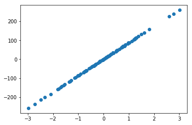
Document description of datasets.make_regression
5. Common attributes and functions in sklearn model
After data training, the model will correspondingly contain different attributes and functions. Next, let's see what attributes and functions are there?
#For the linear regression model, the coefficients and intercepts of the fitting line can be output from the model trained at last.
#At the same time, the parameters used in the training model can be obtained, and the training model can be scored.
from sklearn import datasets
from sklearn.linear_model import LinearRegression  #Importing Linear Regression Model

#Loading data
load_data=datasets.load_boston()
data_X=load_data.data
data_y=load_data.target
print(data_X.shape) #Sample Number and Sample Characteristic Number

#Training data
model=LinearRegression()
model.fit(data_X,data_y)
model.predict(data_X[:4,:])  #Forecast the first four data

#View some properties and functions of the model
w=model.coef_  #Coefficient of fitting straight line
b=model.intercept_  #Interception of Fitted Lines
param=model.get_params() #Model training parameters

print(w)
print(b)
print(param)
(506, 13)
[-1.07170557e-01  4.63952195e-02  2.08602395e-02  2.68856140e+00
 -1.77957587e+01  3.80475246e+00  7.51061703e-04 -1.47575880e+00
  3.05655038e-01 -1.23293463e-02 -9.53463555e-01  9.39251272e-03
 -5.25466633e-01]
36.49110328036181
{'copy_X': True, 'fit_intercept': True, 'n_jobs': 1, 'normalize': False}
For linear regression, as for other models, it is very convenient to view the properties and methods of models according to official documents.
6. Data standardization
In many learning algorithms, the objective function is based on the assumption that all features are zero-mean and have variances of the same order (such as radial basis function, support vector machine and L1L2 regularization term). If the variance of one feature is several orders of magnitude larger than that of other features, then it will dominate the learning algorithm, leading to the neglect of other features by the learner.
Standardization first centralizes the data and then scales it by dividing the standard deviation of features.
In sklearn s, we can Scale data to achieve standardization.
from sklearn import preprocessing
import numpy as np
a=np.array([[10,2.7,3.6],
           [-100,5,-2],
            [120,20,40]],dtype=np.float64)
print("Data before standardization:",a)
print("Standardized data:",preprocessing.scale(a))
Data before standardization: [10.2.7 3.6]
 [-100.     5.    -2. ]
 [ 120.    20.    40. ]]
Standardized data: [0. -0.85170713-0.55138018]
 [-1.22474487 -0.55187146 -0.852133  ]
 [ 1.22474487  1.40357859  1.40351318]]
Next, let's look at the difference between data processing without standardization and data processing with standardization.
from sklearn.model_selection import train_test_split
from sklearn.datasets.samples_generator import make_classification
from sklearn.svm import SVC
import matplotlib.pyplot as plt

#The generated data is visualized as follows
plt.figure()
X,y=make_classification(n_samples=300,n_features=2,n_redundant=0,n_informative=2,
                       random_state=22,n_clusters_per_class=1,scale=100)
plt.scatter(X[:,0],X[:,1],c=y)
plt.show()
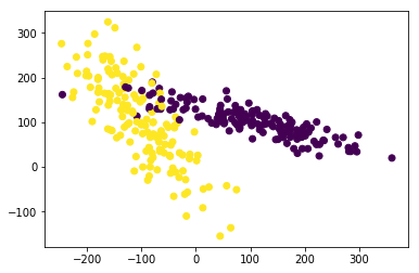
X_pre=X
y_pre=y
X_train_pre,X_test_pre,y_train_pre,y_test_pre=train_test_split(X_pre,y_pre,test_size=0.3)
clf=SVC()
clf.fit(X_train_pre,y_train_pre)
print(clf.score(X_test_pre,y_test_pre))
0.5222222222222223
#Standardization of data by minmax
X=preprocessing.minmax_scale(X) #feature_range=(-1,1)  #Reset range can be set
X_train,X_test,y_train,y_test=train_test_split(X,y,test_size=0.3)
clf=SVC()
clf.fit(X_train,y_train)
print(clf.score(X_test,y_test))
0.9111111111111111
It can be seen that the model score is 0.52222 before data normalization and 0.91111 after data normalization.
7. Test Neural Network
So what are the methods of cross validation? Let's briefly introduce four methods.
8. Cross-validation
The idea of cross-validation is to use data repeatedly, divide the sample data into different training sets and validation sets, train the model with training sets, and evaluate the prediction of the model with validation sets.
(1) Simple cross-validation:
The sample data is randomly divided into two parts (such as 70% training and 30% testing). Then the training set is used to train the model and validate the model and parameters on the validation set. Then the samples are scrambled, the training set and validation set are re-selected, and the validation is re-trained. Finally, the loss function is selected to evaluate the optimal model and parameters.
(2) k-fold cross-validation:
The samples were randomly divided into K samples, and k-1 samples were randomly selected as training set and the remaining one as validation set. When this round is completed, k-1 copies of training data are randomly selected again. After several rounds, loss function is selected to evaluate the optimal model and parameters.
(3) Leave a cross-validation:
Keeping one cross-validation is a special case of k-fold cross-validation. At this time, k = n (the number of samples), n-1 samples are selected for training each time, and one sample is left to verify the model.
This method is suitable for very small sample size.
(4) Boostrapping self-sampling method:
This method is also used in random forest training samples.
In n samples, m samples are randomly put back as a training set of a tree. This adoption will result in about one third of the samples not being collected, and these samples will be used as the verification set of the tree.
If only do a preliminary model of data, do not need to do in-depth analysis, simple cross-validation can be done, otherwise using k-fold cross-validation, in a small sample size, you can choose to use the retention method.
In a word, everything is not the same. When you encounter specific problems, you can try all kinds of ways to see the effect and choose the right method according to the specific problems.
from sklearn.datasets import load_iris
from sklearn.model_selection import train_test_split
from sklearn.neighbors import KNeighborsClassifier
 from sklearn.model_selection import cross_val_score import cross-validation

# Loading data
iris=load_iris()
X=iris.data
y=iris.target

# Training data
X_train,X_test,y_train,y_test=train_test_split(X,y,test_size=0.3)


KNN = KNeighbors Classifier (n_neighbors = 5)# Select five adjacent points
 scores=cross_val_score(knn,X,y,cv=5,scoring='accuracy')#5 fold cross-validation, the scoring method is accuracy.
print(scores)# Score results for each group

Print (scores. mean ()# average score results
[0.96666667 1.         0.93333333 0.96666667 1.        ]
0.9733333333333334
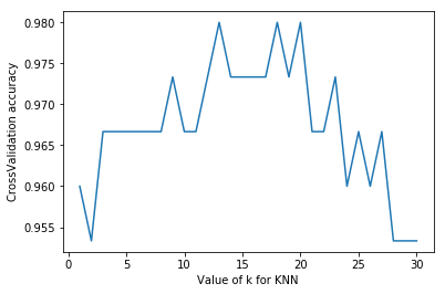
#Adjustment of model parameters by k=5 in k-nearest neighbor method
from sklearn import datasets
from sklearn.model_selection import train_test_split
from sklearn.neighbors import KNeighborsClassifier
from sklearn.model_selection import cross_val_score#Introducing cross validation
import  matplotlib.pyplot as plt
#Loading data
iris=datasets.load_iris()
X=iris.data
y=iris.target
#Set the value of n_neighbors from 1 to 30 to see the training score by drawing
k_range=range(1,31)
k_score=[]
for k in k_range:
    knn=KNeighborsClassifier(n_neighbors=k)
    scores=cross_val_score(knn,X,y,cv=10,scoring='accuracy')#10 fold cross validation
    k_score.append(scores.mean())
plt.figure()
plt.plot(k_range,k_score)
plt.xlabel('Value of k for KNN')
plt.ylabel('CrossValidation accuracy')
plt.show()
#Overfitting is a problem caused by over-fitting. We can choose the value between 12 and 18.

In addition, we can choose 2-fold cross validation,leave-one-out cross validation and other methods to segment data, and compare different methods and parameters to get the optimal results.
# Adjustment of model parameters by k=5 in k-nearest neighbor method
from sklearn import datasets
from sklearn.model_selection import train_test_split
from sklearn.neighbors import KNeighborsClassifier
from sklearn.model_selection import cross_val_score#Introducing cross validation
# from sklearn.model_selection import LeaveOneOut
import  matplotlib.pyplot as plt
#Loading data
iris=datasets.load_iris()
X=iris.data
y=iris.target
print(len(X))

#Set the value of n_neighbors from 1 to 30 to see the training score by drawing
k_range=range(1,31)
k_score=[]
for k in k_range:
    knn=KNeighborsClassifier(n_neighbors=k)
    scores=cross_val_score(knn,X,y,cv=10,scoring='accuracy')#10 fold cross validation
    k_score.append(scores.mean())
plt.figure()
plt.plot(k_range,k_score)
plt.xlabel('Value of k for KNN')
plt.ylabel('CrossValidation accuracy')
plt.show()
150
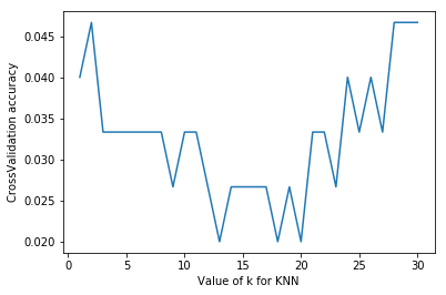
#Change the scoring function "neg_mean_squared_error"
from sklearn import datasets
from sklearn.model_selection import train_test_split
from sklearn.neighbors import KNeighborsClassifier
from sklearn.model_selection import cross_val_score#Introducing cross validation
# from sklearn.model_selection import LeaveOneOut
import  matplotlib.pyplot as plt
#Loading data
iris=datasets.load_iris()
X=iris.data
y=iris.target
print(len(X))

#Set the value of n_neighbors from 1 to 30 to see the training score by drawing
k_range=range(1,31)
k_score=[]
for k in k_range:
    knn=KNeighborsClassifier(n_neighbors=k)
    loss=-cross_val_score(knn,X,y,cv=10,scoring='neg_mean_squared_error')#10 fold cross validation
    k_score.append(loss.mean())
plt.figure()
plt.plot(k_range,k_score)
plt.xlabel('Value of k for KNN')
plt.ylabel('CrossValidation accuracy')
plt.show()
150
8. Overfitting
The problem of over-fitting is that the model is too complex to fit the training data well, but it can not deal with the test data correctly. From one point of view, it learns some non-general information about the sample data. It makes the generalization effect of the model very bad.
# How to Identify overfitting Problem by First Distance
# The learning curve in Sklearn.learning_curve can intuitively see the progress of model learning, and compare whether it has been fitted or not.
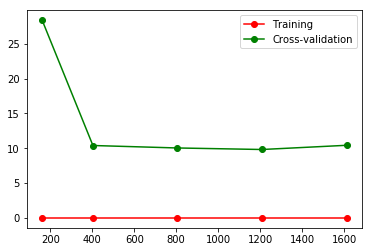
from sklearn.model_selection import learning_curve  # learning curve
from sklearn.datasets import load_digits
from sklearn.svm import SVC
import matplotlib.pyplot as plt
import numpy as np

#Loading data
digits=load_digits()
X=digits.data
y=digits.target

#train_size means recording a step in the learning process, such as 10%, 25%...
train_size,train_loss,test_loss=learning_curve(
    SVC(gamma=0.1),X,y,cv=10,scoring='neg_mean_squared_error',
    train_sizes=[0.1,0.25,0.5,0.75,1]
)
train_loss_mean=-np.mean(train_loss,axis=1)
test_loss_mean=-np.mean(test_loss,axis=1)

plt.figure()
#Print out each step
plt.plot(train_size,train_loss_mean,'o-',color='r',label='Training')
plt.plot(train_size,test_loss_mean,'o-',color='g',label='Cross-validation')
plt.legend(loc='best')
plt.show()
# If the value of the loss function stays around 10, the fitting can be seen intuitively.
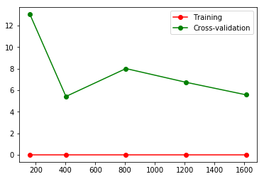
#Changing the gamma value of 0.01 will change the loss function accordingly.
from sklearn.model_selection import learning_curve  # learning curve
from sklearn.datasets import load_digits
from sklearn.svm import SVC
import matplotlib.pyplot as plt
import numpy as np

#Loading data
digits=load_digits()
X=digits.data
y=digits.target

#train_size means recording a step in the learning process, such as 10%, 25%...
train_size,train_loss,test_loss=learning_curve(
    SVC(gamma=0.01),X,y,cv=10,scoring='neg_mean_squared_error',
    train_sizes=[0.1,0.25,0.5,0.75,1]
)
train_loss_mean=-np.mean(train_loss,axis=1)
test_loss_mean=-np.mean(test_loss,axis=1)

plt.figure()
#Print out each step
plt.plot(train_size,train_loss_mean,'o-',color='r',label='Training')
plt.plot(train_size,test_loss_mean,'o-',color='g',label='Cross-validation')
plt.legend(loc='best')
plt.show()
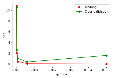
# The change of Loss function can be seen by changing different gamma values.
from sklearn.model_selection import validation_curve  # Verification curve
from sklearn.datasets import load_digits
from sklearn.svm import SVC
import matplotlib.pyplot as plt
import numpy as np

#Loading data
digits=load_digits()
X=digits.data
y=digits.target

#Change param to observe loss function
param_range=np.logspace(-6,-2.3,5)
train_loss,test_loss=validation_curve(
    SVC(),X,y,param_name='gamma',param_range=param_range,cv=10,
    scoring='neg_mean_squared_error'
)
train_loss_mean=-np.mean(train_loss,axis=1)
test_loss_mean=-np.mean(test_loss,axis=1)

plt.figure()
plt.plot(param_range,train_loss_mean,'o-',color='r',label='Training')
plt.plot(param_range,test_loss_mean,'o-',color='g',label='Cross-validation')
plt.xlabel('gamma')
plt.ylabel('loss')
plt.legend(loc='best')
plt.show()
9. Save the model
We spend a lot of time training data, adjusting parameters and getting the optimal model. But if we change the platform, we need to retrain the data and modify the parameters to get the model, which will be a waste of time. At this point, we can save the model first, and then we can easily migrate the model.
from sklearn import svm
from sklearn import datasets

#Loading data
iris=datasets.load_iris()
X,y=iris.data,iris.target
clf=svm.SVC()
clf.fit(X,y)

print(clf.get_params)
<bound method BaseEstimator.get_params of SVC(C=1.0, cache_size=200, class_weight=None, coef0=0.0,
  decision_function_shape='ovr', degree=3, gamma='auto', kernel='rbf',
  max_iter=-1, probability=False, random_state=None, shrinking=True,
  tol=0.001, verbose=False)>
#Import the Save Module in sklearn
from sklearn.externals import joblib

#Save the model
joblib.dump(clf,'sklearn_save/clf.pkl')
['sklearn_save/clf.pkl']
#Reload the model, which can only be loaded after saving it once
clf3=joblib.load('sklearn_save/clf.pkl')
print(clf3.predict(X[0:1]))
#Save the model to get previous results faster
[0]
Sklearns have a lot of knowledge and are used in practice. Above all, we have only explained some knowledge points. First, we are familiar with what sklearns can do and how to use it. If you want to know sklearns in more detail, you may want to see the explanation in the official documents.
sklearn User Guidance
Summary
For machine learning tasks, generally our main steps are:
1. Loading data sets (your own data, or online data, or sklearn s own data)
2. Data preprocessing (dimensionality reduction, data normalization, feature extraction, feature transformation)
3. Select the model and train it. (Look directly at the api to find the method you need, call it directly, and you may need to adjust parameters, etc.)
4. Model scoring (using the score method of the model itself, or using sklearn index function, or using its own evaluation method)
5. Model preservation
sklearn's Classification Algorithms
Scikit-learn ing is a free software machine learning library for Python programming language. It has a variety of classification, regression and clustering algorithms, including support vector machines, random forests, gradient enhancement, K-means and DBSCAN, designed to interoperate with Python numerical and scientific libraries Numpy and Scippy. Below we learn the machine learning classification algorithm in sklearn s - Logical Regression, Naive Bayesian, KNN, SVM, Decision Tree.