Note: This paper only makes a simple quantitative analysis of the stock data through its own knowledge, only considering the closing situation. It is not enough to only consider the closing situation in the real quantitative trading, there are many complex factors, and only three years of data is not enough to guide the real stock trading, so this paper is just as a simple python practice Eye.
I. analysis purpose
Using the pre-set strategy, through the backtesting of the historical data of stock trading, to verify whether the strategy can guide stock trading.
II. Data processing
1. Data set description
Data set source: https://www.nasdaq.com/symbol/baba/historical
Data set introduction: this data set is from the Nasdaq website, and the data obtained in this paper is from 2016 / 04 / 15 to 2019 / 04 / 15.
Column name understanding:
The field and column names of the original data table are very standard and do not need to be renamed. The following is the understanding of each column name:
Date: date
close: closing price
Volume: Volume
open: opening price
high: daily maximum price
low: daily minimum price
This time, it is only a simple analysis of the closing price.
2. Data cleaning
The dataset is relatively standard, there are no duplicate values and its exception values need to be handled.
3. Data import
# Loading Library
import numpy as np
import pandas as pd
# Load data (only date and closing price are used this time)
df = pd.read_csv('E:/Related folders/BABA_stock.csv',index_col = 'date',usecols = [0,1])
df.head()

3. Data analysis
# Convert index to date index
df.index = pd.to_datetime(df.index)
# df.index = pd.DatetimeIndex(df.index.str.strip("'"))
df.index
# Sort by index
df.sort_index(inplace = True )
df.head()

Buying and selling strategy: buy when the day before is lower than the 60 day average and buy when the day after is higher than the 60 day average, and sell when the day before is higher than the 60 day average and the day after is lower than the 60 day average.
1. Calculate the 60 day moving average
ma60 = df.rolling(60).mean().dropna()
ma60
2. Buy when find value changes from False to True, and sell when True changes to False
ma60_model = df['close'] - ma60['close'] >0
ma60_model
3. Find out the buying and selling points
# Customize the way to find the buying and selling points
def get_deal_date(w,is_buy = True):
    if is_buy == True:
        return True if w[0] == False and w[1] == True else False
    else:
        return True if w[0] == True and w[1] == False else False
# raw=False if not, there will be a warning message
# If the Na value is deleted, there will be missing, so fill it with 0 here, and convert it to bool value for later value
se_buy = ma60_model.rolling(2).apply(get_deal_date,raw = False).fillna(0).astype('bool')
se_buy
# apply's args accepts an array or dictionary to pass parameters to a custom function
se_sale = ma60_model.rolling(2).apply(get_deal_date,raw = False,args = [False]).fillna(0).astype('bool')
se_sale


# Using Boolean index to find out the buying and selling points
buy_info = df[se_buy.values]
sale_info = df[se_sale.values]
buy_info
sale_info
4. Calculation of profit (trading profit per share)
# Convert to numeric index: the index needs to be processed before operation
no_index_buy_info = buy_info.reset_index(drop = True)
no_index_sale_info = sale_info.reset_index(drop = True)
print(no_index_buy_info.head())
print(no_index_sale_info.head())
# Profit situation
profit = no_index_sale_info - no_index_buy_info
# There is no selling point in the last set of data, and a null value may appear
profit.dropna()

# Calculate the overall profit
profit.describe()
# How much did you make in all
profit.sum()
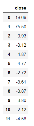

Figure a figure b
close    57.66
dtype: float64
It can be seen from figure a that there are profits and losses in every purchase and sale. From the overall situation of figure b, there are 12 transactions in total, with the most losses of $8.61, with an average profit of $4.8 each time, and the most losses of $75.5 each time. Through the analysis of
The total profit of all transactions is 57.66 US dollars, which is profitable in general.
5. Final profit of USD 1w
Strategy: put the money from each sale into the next purchase
all_money = 10000
remain = all_money
# If you add the handling fee of 3 / 10000 of each transaction amount
fee = 0.0003
# Since the last time there is no selling point, the number of transactions needs to be reduced by one from the number of purchases
for i in range(len(no_index_buy_info)-1):
    buy_count = remain/no_index_buy_info.iloc[i]
    remain = buy_count * no_index_sale_info.iloc[i]*(1-fee)
    print(remain)
close    12413.412104
Name: 0, dtype: float64
close    22301.278558
dtype: float64
close    22412.294488
dtype: float64
close    22024.926199
dtype: float64
close    21439.23349
dtype: float64
close    20885.390796
dtype: float64
close    20576.028522
dtype: float64
close    19640.163023
dtype: float64
close    19232.001776
dtype: float64
close    18857.206606
dtype: float64
close    18595.722503
dtype: float64
close    18044.391215
dtype: float64
It can be seen from the above results that: the profit obtained in three years is 8044.39 US dollars, with an annualized rate of about 26%, and the overall income is still very good. This strategy can be put into other cycles or other stocks for analysis. If all the profits can be made, it shows that this strategy is effective in guiding stock trading.