Decision tree algorithm type
Decision tree is a series of algorithms, not an algorithm.
The decision tree includes ID3 classification algorithm, C4.5 Classification Algorithm, Cart classification tree algorithm and Cart regression tree algorithm.
Decision tree can be used as both classification algorithm and regression algorithm. Therefore, decision tree can solve both classification problem and regression problem.
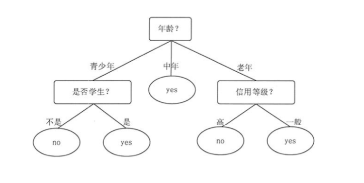
Generally speaking, in the decision tree, the root node and sub node are represented by squares, while the leaf node is represented by ellipses.
The key point of decision tree is how to build a tree and how to build a tree with the shallowest depth on the premise that the goal can be achieved
Introduction of different algorithms in decision tree
CLS, ID3, C4.5 and CART, of which ID3, C4.5 and CART all adopt greedy method, in which the decision tree is constructed by top-down recursive divide and conquer method, and most decision tree algorithms adopt this top-down method. The so-called greedy method, popularly speaking, is to calculate all when selecting the root node, and use the exhaustive method to find the best
Introduction to CLS algorithm
CLS is the earliest decision tree algorithm. It does not give how to determine the root node, but gives the specific method to create the decision tree. The other three algorithms are the optimization and extension of CLS.
Basic process of CLS:
- Generate an empty decision tree and a training set sample attribute set.
- If all samples in the training set belong to the same class, a leaf node is generated to terminate the algorithm.
- According to a certain strategy, select attributes from the attributes of training set samples as split attributes to generate test nodes.
- It is divided into different branches according to the value of the test node.
- Delete the split attributes from the attributes of the training sample.
- Turn to step 2 and repeat the operation until all the split data belong to the same class.
Generally speaking:
CLS is to randomly select a column from the dataset (equivalent to a feature or an attribute). If all its values belong to the same category, it will terminate. Otherwise, delete the column, and then split according to the value branches of the deleted column until all splits belong to the same category.
Introduction to ID3 classification algorithm
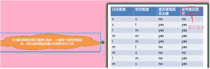
ID3 mainly aims at attribute selection, and uses information gain degree to select split attributes.
characteristic:
1. Only classification algorithm can be implemented.
2. Information gain is used as the evaluation criterion of splitting attribute.
3. The feature must be discrete data.
4. The tree can have multiple branches (multi fork tree), that is, a feature attribute can have multiple values, and each value is a branch.
5. Multi classification algorithm (the value of label can be greater than 2)
Disadvantages:
The features with multiple attribute values are preferentially selected for splitting
What is information gain entropy?
Calculation formula of information quantity: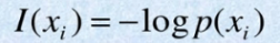
The greater the probability of information occurrence, the less information it has, that is, the smaller the probability of occurrence, the greater the amount of information. For example, when the probability is equal to 1, the amount of information is equal to - log(1)
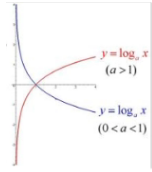
In information theory, the index is usually based on 2, so only the red line in the figure needs to be considered.
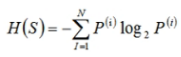
The understanding of entropy can be simplified to weighted average information. There are N values of feature S, and the probability of each possible occurrence multiplied by its information and added together is the weighted average information.
Conditional entropy
Equivalent to conditional probability
1. Calculate the entropy of the result first.
2. Calculate the entropy of the result under a known characteristic condition.
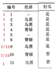
give an example:
Suppose there are three values for a feature and two values for a tag.
1. First calculate the probability of three values of the feature: P1, P2 and P3
2. Calculate the entropy of the result under each value.
3. Conditional entropy = weighted average of three entropy values under three value results.
information gain
The function of information gain is to determine the characteristics as the root node. The calculation formula of conditional entropy of the result under the condition of subtracting the known characteristics from the entropy of the result:
Gain (characteristic) = H (result) - H (result | characteristic)
Conclusion: the root node with the largest information gain is selected
Summary:
1. Suppose there is a dataset containing several features and one label.
2. Calculate the result entropy for the label.
3. Calculate the conditional entropy of the corresponding results for the values in all features.
4. Calculate the information gain of each feature and select the maximum value as the root node.
5. Delete the split feature column. If the result is the same class, end the algorithm.
6. If it is not the same class, continue to calculate the information gain of the remaining features, and select the largest feature as the feature of the next split.
7. Repeatedly calculate the information gain and select the feature to split until all leaf nodes are of the same class.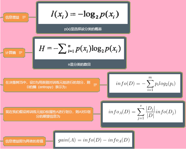

Introduction to C4.5 Classification Algorithm
Some optimizations are made on the basis of ID3. By using the information gain rate to select split attributes, the defect that ID3 algorithm can not process many attribute values through information gain is overcome. The information gain rate can process discrete data and continuous data, as well as training data with real attributes.
Information gain rate
The information gain rate can effectively avoid the tendency to choose samples with multiple attribute values
Information gain rate formula:
Gainraio = gain / h
Select the feature with the largest gain rate as the root node, and the use process is the same as that of information gain
Continuous value processing
For the processing of continuous data, the information gain rate processing is no longer used, but the following method is used:
1. Suppose there are N continuous data in a feature.
2. Sort this column of data in ascending order after de duplication.
3. Calculate the mean value of two adjacent values, so that N-1 data can be obtained.
4. First, use the first data to calculate the conditional entropy less than the value of the first data and the conditional entropy greater than the first data, and then calculate the information gain of the data.
5. Calculate the information gain of the remaining N-2 data.
6. When comparing the information gain, select the attribute value corresponding to the maximum information gain as the splitting point (for example, if there is a column with the feature of density, when the density = 0.318, the information gain is the maximum, select this point as the splitting point, and its value will become two types less than 0.318 and greater than or equal to 0.318, and then split)
summary
The information gain rate can deal with the characteristics of particularly many attribute values; Discrete data will be deleted after splitting, but the data after continuous value processing will not be deleted after splitting, and can be used as attribute division in the future.
shortcoming
Through the above processing, only the continuous features can be dichotomized, and still only the classification algorithm can be realized. The following algorithm has been improved to realize the processing classification algorithm and regression algorithm.
CART algorithm
CART can implement Classification and regression algorithms. sklearn includes Classification and Regression Tree respectively
Characteristics of CART algorithm
Gini coefficient is used in the classification algorithm as the evaluation standard of splitting attribute.
The average error is used in the regression algorithm as the evaluation standard of splitting attribute.
A tree is a binary tree.
Multi classification algorithm
Relationship between Gini and entropy: the trend of Gini and entropy is the same, and Gini also becomes half of entropy, so the operation of Gini is simpler.
Gini coefficient
Gini coefficient formula: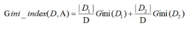
Gini value represents the impurity of the model. The smaller the Gini value, the lower the impurity and the better the characteristics. Gini value = probability that the sample is selected - probability that the sample is misclassified, expressed as 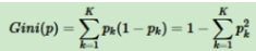
Gini coefficient is for two categories, which will only be divided into yes or no. For a feature, all values in the feature should calculate the Gini value of the corresponding result, then calculate the Gini coefficient, and select the smallest as the splitting node
Gini coefficient can only be used in classification algorithm
Square error
The binary regression algorithm is used to calculate the square error to process the continuous labels. The specific steps are as follows:
1. Firstly, several values of a feature are selected for calculation, which is similar to conditional entropy. When the value is known, the average error of the result.
2. Select the one with small average error as the splitting node.
3. If the left node is less than or equal to three, the splitting of the left subtree will be terminated. If it is greater than 3, the transformation coefficient of the node will continue to be judged. If it is less than 0.1, the splitting of the left subtree will be stopped. Otherwise, the splitting will continue, and the same is true for the right subtree.
4. Delete the split features and continue to judge which of the remaining features has the smallest average error.
5. Stop until the transformation coefficient is less than 0.1 or the number of rows is less than 3. If the label still has more than two values when stopping, take its mean value as the result.
Square error calculation process:
Because it is a secondary classification, it is only divided into yes and No. the average error calculated if it is classified as yes plus the average error classified as no is the average error of the node. The formula of average error is: (X - X mean) * * 2, which can also be called N-th variance.
Transform coefficient: also known as discrete coefficient or variation coefficient. The discrete coefficient is equal to the standard deviation divided by the mean, but the average error divided by the mean when used in the average error.
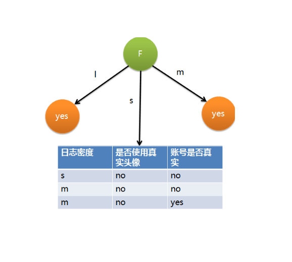
Missing value processing
Weight is the most used in missing value processing. Take information gain as an example:
1. For example, if a feature has missing values, when calculating the information gain of the column, first remove the rows with missing values and calculate the information gain of the remaining rows
2. Missing values of other features are also calculated in this way
3. By comparing the calculated information gain, select the largest as the root node, but this is only the method of selecting the root node
4. After selecting the root node, split it according to the value
5. For example, the root node column has two missing values and is divided into three branches. The number of data on each branch is 7, 5 and 3 respectively; At this time, the missing value should be added back, because the row corresponding to the missing value still has result information, and subsequent selection needs to be used. Two missing values should be added to each branch, and the data on the three branches will become 9, 7 and 5;
6. The weight of each row of data is 1, but the missing value is different, because there are 7, 5 and 3 missing data on each branch; The weight of two missing values becomes: the number of branch data / (7 + 5 + 3 + 2), that is, 7 / 15, 5 / 15 and 3 / 15. The weight of no missing value is still 1
7. After calculating the information gain of the remaining features respectively according to the weight and removing the missing value of the feature to be calculated, first calculate the entropy of the result, H (result) = - p1log(p1) - p2log(p2). The probability P in the formula needs to be calculated according to the weight, P = non missing value weight / total weight, p1 = (4 + 7/15) / (5 + 2 * 7/15). The calculation of conditional entropy is the same, Then select the one with the largest information gain to split and repeat the process of weighting calculation
The processing of missing values is still troublesome. When there is enough data, it is recommended to delete the missing rows directly
Implementation of decision tree based on sklearn
Characteristics of decision tree
Split using perpendicular to eigenvalues
Tree structure can be generated with good visualization effect [0 basic people can understand the algorithm prediction process]
No standardization required
Attributes that do not contribute to the goal can be automatically ignored
Implementation of decision tree classification tree based on sklearn
import pandas as pd
from sklearn.model_selection import train_test_split
#Classification tree
from sklearn.tree import DecisionTreeClassifier

#Reading of data set
work_data=pd.read_csv('./HR_comma_sep.csv')
work_data['department1']=work_data['department'].astype('category').cat.codes
work_data['salary1']=work_data['salary'].astype('category').cat.codes
x=work_data[['satisfaction_level', 'last_evaluation', 'number_project','average_montly_hours', 'time_spend_company', 'Work_accident','promotion_last_5years', 'department1','salary1']]
y=work_data['left']

#Data splitting
X_train, X_test, y_train, y_test = train_test_split(
    x,  # features
    y,  # label
    test_size=0.2,  # How much data is allocated to the test set
    random_state=1,
    stratify=y,  # Layering ensures that the proportion of each category is consistent before and after splitting
)

#Decision tree
start_time=time.time()
dt = DecisionTreeClassifier()
dt.fit(X_train,y_train)
print("Decision tree prediction accuracy", dt.score(X_test, y_test))
end_time=time.time()
print("Decision tree time", end_time-start_time)
Implementation of decision tree regression tree based on sklearn
import pandas as pd
from sklearn.model_selection import train_test_split
#Regression tree
from sklearn.tree import DecisionTreeRegressor
#Data acquisition
selery_data=pd.read_excel('./job.xlsx',sheet_name=1)
name = selery_data['language'].astype("category").cat.categories
selery_data['Language 1']=selery_data['language'].astype("category").cat.codes
selery_data['Education 1']=selery_data['education'].astype("category").cat.codes
x1=selery_data[['Language 1','hands-on background(year)','Education 1']].values
y1=selery_data['Maximum salary(element)'].values
#Splitting of data
X_train1, X_test1, y_train1, y_test1 = train_test_split(
    x1,  # features
    y1,  # label
    test_size=0.2,  # How much data is allocated to the test set
    random_state=1,
    # stratify=y1,  # Layering ensures that the proportion of each category is consistent before and after splitting
)
#Regression tree
dt=DecisionTreeRegressor()
alg.fit(X_train1, y_train1)
print("Regression tree accuracy", alg.score(X_test1, y_test1))
Search for optimal parameters of decision tree
import pandas as pd
from sklearn.model_selection import train_test_split
#Classification tree
from sklearn.tree import DecisionTreeClassifier
#Grid search
from sklearn.model_selection import GridSearchCV

#Reading of data set
work_data=pd.read_csv('./HR_comma_sep.csv')
work_data['department1']=work_data['department'].astype('category').cat.codes
work_data['salary1']=work_data['salary'].astype('category').cat.codes
x=work_data[['satisfaction_level', 'last_evaluation', 'number_project','average_montly_hours', 'time_spend_company', 'Work_accident','promotion_last_5years', 'department1','salary1']]
y=work_data['left']

#Data splitting
X_train, X_test, y_train, y_test = train_test_split(
    x,  # features
    y,  # label
    test_size=0.2,  # How much data is allocated to the test set
    random_state=1,
    stratify=y,  # Layering ensures that the proportion of each category is consistent before and after splitting
)
#Exploration on optimal parameters of grid search
dt = DecisionTreeClassifier()
param_grid = {"criterion": ["gini", "entropy"], "max_depth": [3, 5, 6, 7, 9]}
gird = GridSearchCV(dt, param_grid)
gird.fit(X_train, y_train)
print("Best parameters", gird.best_params_)

#Cross validation to explore the optimal parameters
from sklearn.model_selection import cross_val_score
for max_depth in [3, 5, 6, 7, 9]:
    for criterion in ["gini", "entropy"]:
        dt = DecisionTreeClassifier(max_depth=max_depth, criterion=criterion)
        score = cross_val_score(dt, X_train, y_train, cv=5).mean()
        # print(score)
        print("Depth is{} criterion{} The score is{}".format(max_depth, criterion, score))


#Classification tree
start_time=time.time()
dt = DecisionTreeClassifier()
dt.fit(X_train,y_train)
print("Decision tree prediction accuracy", dt.score(X_test, y_test))
end_time=time.time()
print("Decision tree time", end_time-start_time))
Decision tree output tree
# Export algorithm model dt to dot file
from sklearn.tree import export_graphviz
export_graphviz(dt, 'titanic.dot',
                feature_names=["pclass", "age", "sex"],
                feature_names=["shipping space", "Age", "Gender"],
                max_depth=5,  # Depth of tree
                class_names=['death', 'existence']  # Category name
)

#Use the following command to convert the generated titanic.dot to picture format
# dot -Tpng tree.dot -o tree.png