1, Multiple linear regression

The changes of socio-economic phenomena are often affected by multiple factors. Therefore, multiple regression analysis is generally required. We call the regression including two or more independent variables as multiple linear regression.
The basic principle and calculation process of multiple linear regression are the same as that of univariate linear regression, but due to the large number of independent variables, the calculation is quite troublesome. Generally, statistical software should be used in practical application. This paper only introduces some basic problems of multiple linear regression.
However, the units of each independent variable may be different. For example, in a consumption level formula, factors such as wage level, education level, occupation, region and family burden will affect the consumption level, and the units of these influencing factors (independent variables) are obviously different. Therefore, the size of the coefficient before the independent variable does not explain the importance of this factor, More simply, for the same wage income, the regression coefficient obtained by using yuan as the unit is smaller than that obtained by using 100 yuan as the unit, but the impact of wage level on consumption has not changed, so we have to find a way to quantify each self variable to a unified unit. The standard score learned earlier has this function. Specifically, it is to convert all variables, including dependent variables, into standard scores first, and then conduct linear regression. At this time, the regression coefficient can reflect the importance of the corresponding independent variable. The regression equation at this time is called the standard regression equation, and the regression coefficient is called the standard regression coefficient, which is expressed as follows:

Since they are converted into standard scores, there is no constant term a, because when each variable takes the average level, the dependent variable should also take the average level, and the average level just corresponds to the standard score 0. When the variables at both ends of the equation take 0, the constant term will be 0.
Multivariate linear regression is similar to univariate linear regression. The model parameters can be estimated by the least square method, and the model and model parameters need to be statistically tested.
Selecting appropriate independent variables is one of the prerequisites for correct multiple regression prediction. The selection of independent variables in multiple regression model can be solved by using the correlation matrix between variables.

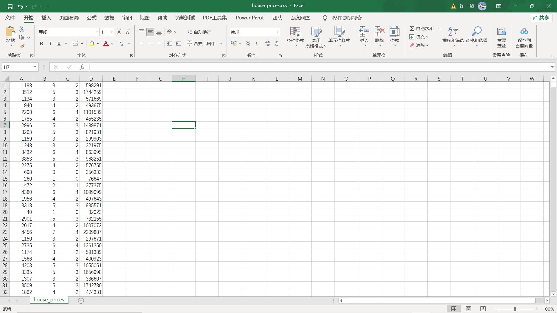
2, Using excel to estimate house prices

1. Open the dataset file and delete non data items to facilitate multiple linear regression

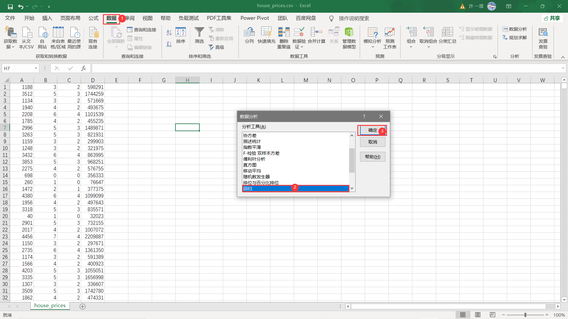
2. Selective regression data analysis

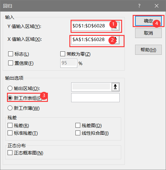
3. Select a dataset and export the results

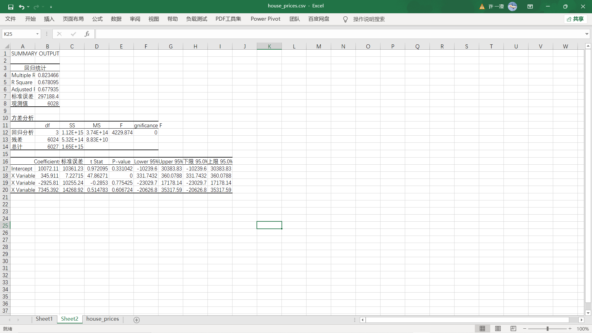
4. Results

3, Estimated house price in python (with the help of sklearn Library)

1. Upload dataset to jupyter

2. Import package

import pandas as pd
import numpy as np
import seaborn as sns
from sklearn import datasets
from sklearn.linear_model import LinearRegression
from statsmodels.formula.api import ols

3. Read dataset data

df = pd.read_csv('house_prices.csv')
df.info()#Displays column names and data types
df.head(6)#The first n lines are displayed, and N defaults to 5

4. Fetch data

#Fetch argument
data_x=df[['area','bedrooms','bathrooms']]
data_y=df['price']

5. Multiple linear regression was carried out and the results were obtained

# Multiple linear regression
model=LinearRegression()
l_model=model.fit(data_x,data_y)
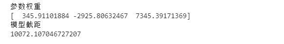
print('Parameter weight')
print(model.coef_)
print('Model intercept')
print(model.intercept_)

result:

• Data processing
  1. Outlier detection

# Outlier handling
# ================Outlier test function: two methods of IQR & Z score=========================
def outlier_test(data, column, method=None, z=2):
    """ Based on a column, the upper and lower truncation point method is used to detect outliers(Indexes) """
    """ 
    full_data: Complete data
    column: full_data Specified line in, format 'x' Quoted
    return Optional; outlier: Outlier data frame 
    upper: Upper truncation point;  lower: Lower truncation point
    method: Method of checking outliers (optional), default None Is the upper and lower cut-off point method),
            choose Z Method, Z The default is 2
    """
    # ==================Upper and lower cut-off point method to test outliers==============================
    if method == None:
        print(f'with {column} Based on the column, the upper and lower cut-off point method is used(iqr) Detect outliers...')
        print('=' * 70)
        # Quartile; There will be exceptions when calling the function here
        column_iqr = np.quantile(data[column], 0.75) - np.quantile(data[column], 0.25)
        # 1, 3 quantiles
        (q1, q3) = np.quantile(data[column], 0.25), np.quantile(data[column], 0.75)
        # Calculate upper and lower cutoff points
        upper, lower = (q3 + 1.5 * column_iqr), (q1 - 1.5 * column_iqr)
        # Detect outliers
        outlier = data[(data[column] <= lower) | (data[column] >= upper)]
        print(f'First quantile: {q1}, Third quantile:{q3}, Interquartile range:{column_iqr}')
        print(f"Upper cutoff point:{upper}, Lower cutoff point:{lower}")
        return outlier, upper, lower
    # =====================Z-score test outliers==========================
    if method == 'z':
        """ Based on a column, the incoming data is the same as the data you want to segment z Score point, return the outlier index and the data frame """
        """ 
        params
        data: Complete data
        column: Specified detection column
        z: Z Quantile, The default is 2, according to z fraction-According to the normal curve table, take 2 at the left and right ends%，
           According to you z Positive and negative setting of scores. It can also be changed arbitrarily to know the data set of any top percentage
        """
        print(f'with {column} List as basis, use Z Fractional method, z Quantile extraction {z} To detect outliers...')
        print('=' * 70)
        # Calculate the numerical points of the two Z fractions
        mean, std = np.mean(data[column]), np.std(data[column])
        upper, lower = (mean + z * std), (mean - z * std)
        print(f"take {z} individual Z Score: greater than {upper} Or less than {lower} Is considered an outlier.")
        print('=' * 70)
        # Detect outliers
        outlier = data[(data[column] <= lower) | (data[column] >= upper)]
        return outlier, upper, lower

2. Get the exception set and discard it

outlier, upper, lower = outlier_test(data=df, column='price', method='z')#Get exception data
outlier.info(); outlier.sample(5)
df.drop(index=outlier.index, inplace=True)#Discard exception data

3. Fetch variable

#Fetch argument
data_x=df[['area','bedrooms','bathrooms']]
data_y=df['price']

4. Multiple linear regression was performed and the results were obtained

# Multiple linear regression
model=LinearRegression()
l_model=model.fit(data_x,data_y)
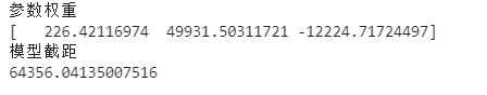
print('Parameter weight')
print(model.coef_)
print('Model intercept')
print(model.intercept_)

result:

3, Linear regression based on statistical analysis library statsmodels

1. Do not use dummy variables
The statsmodels library has been imported earlier. We need to make the necessary packages. Here we start writing directly

#Do not use dummy variables
lm = ols('price ~ area + bedrooms + bathrooms', data=df).fit()
lm.summary()

result:

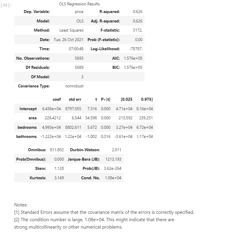
It can be seen that without setting the virtual variable, the correlation coefficient R here is only 0.626. In order to improve the correlation coefficient, we need to set the virtual variable.
2. Set dummy variables and then perform linear regression

# Set dummy variable
# Take the nominal variable neighborhood as an example
nominal_data = df['neighborhood']

# Set dummy variable
dummies = pd.get_dummies(nominal_data)
dummies.sample()  # pandas will automatically name it for you

# One dummy variable generated by each nominal variable needs to be discarded. Here, take discarding C as an example
dummies.drop(columns=['C'], inplace=True)
dummies.sample()
# Splice the results with the original data set
results = pd.concat(objs=[df, dummies], axis='columns')  # Merge by column
results.sample(3)
# You can try to handle the nominal variable style by yourself
# Modeling again
lm = ols('price ~ area + bedrooms + bathrooms + A + B', data=results).fit()
lm.summary()

result:

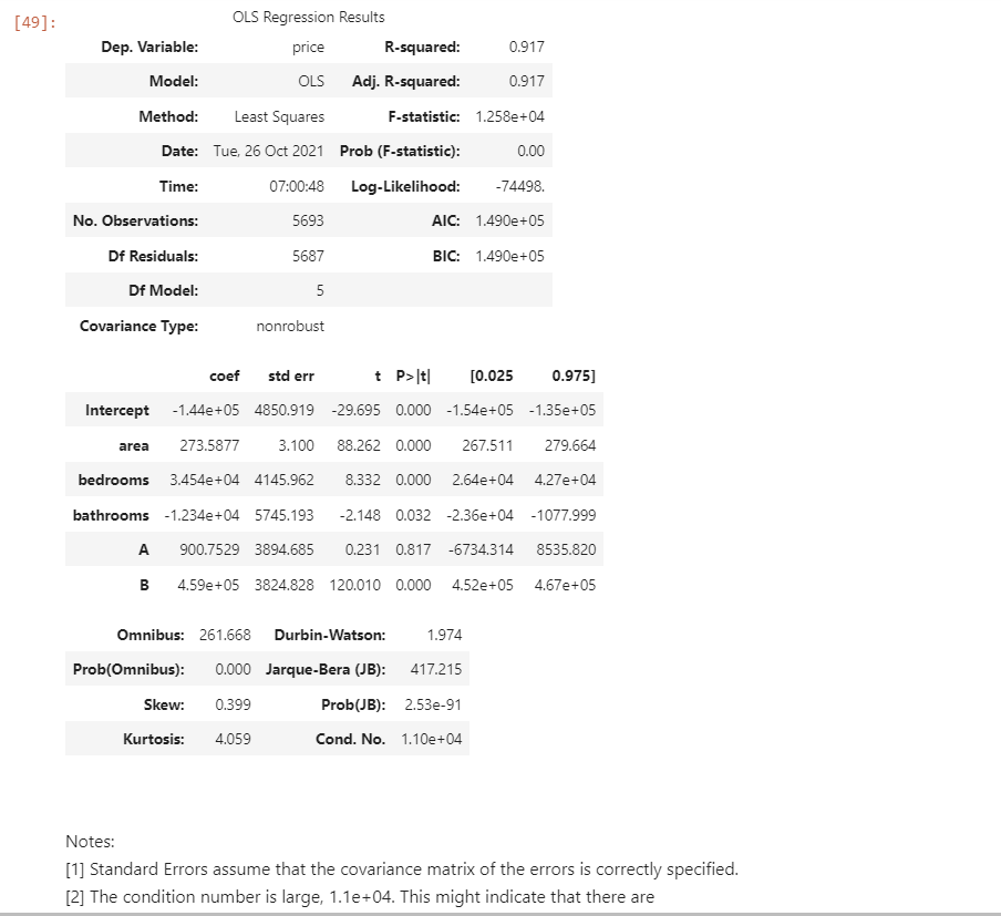
It can be seen that the correlation coefficient has increased to 0.917, but the following note reminds that there may be multicollinearity, so it needs to be tested
3. Detection of multicollinearity factor

# Self defined variance expansion factor detection formula
def vif(df, col_i):
    """
    df: Whole data
    col_i: Detected column name
    """
    cols = list(df.columns)
    cols.remove(col_i)
    cols_noti = cols
    formula = col_i + '~' + '+'.join(cols_noti)
    r2 = ols(formula, df).fit().rsquared
    return 1. / (1. - r2)
    test_data = results[['area', 'bedrooms', 'bathrooms', 'A', 'B']]
for i in test_data.columns:
    print(i, '\t', vif(df=test_data, col_i=i))

result:

It can be seen that bedroom and bathroom are highly correlated
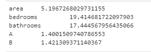
4. Eliminate multiple collinearity, and then carry out linear regression

# It is found that there is a strong correlation between bedrooms and bathrooms, which may explain the same problem
# Sure enough, the variance expansion factors of bedrooms and bathrooms are high,
 # It also confirms the principle that most variance expansion factors appear in pairs. Here, we can discard the bedrooms with large expansion factors
lm = ols(formula='price ~ area + bathrooms + A + B', data=results).fit()
lm.summary()

result:

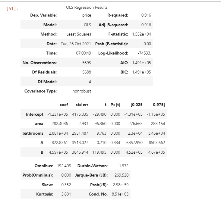
You can see that the value of R has decreased by 0.01

4, Result analysis

When data processing is not performed, the results obtained with excel are the same as those obtained with Python programming, but the results obtained after data cleaning become very different, and the elimination of collinearity also makes the results more reliable.

5, References

Prediction of house prices by jupyter multiple linear regression algorithm
Multiple linear regression analysis
Multiple linear regression algorithm