Common methods to prevent over fitting of neural networks include:

1. Reduce network capacity; 2. Add weight regularization; 3. Add dropout; 4. Get more training data.

Overfitting and underfitting

Over fitting and under fitting

In order to prevent the model from learning wrong or irrelevant patterns from the training data, the best solution is to obtain more training data. The more training data of the model, the better the generalization ability. If more data cannot be obtained, the suboptimal solution is to adjust the amount of information allowed to be stored by the model, or restrict the information allowed to be stored by the model. If a network can only remember a few patterns, the optimization process will force the model to focus on the most important patterns, which is more likely to be well generalized.

This method of reducing over fitting is called regularization. Let's first introduce some of the most common regularization methods:   Then it is applied to practice to improve the film classification model in the previous section.

from keras.datasets import imdb
import numpy as np
​
(train_data, train_labels), (test_data, test_labels) = imdb.load_data(num_words=10000)
​
def vectorize_sequences(sequences, dimension=10000):
    # Create an all zero matrix of shape (len(sequences), dimension)
    results = np.zeros((len(sequences), dimension))
    for i, sequence in enumerate(sequences):
        results[i, sequence] = 1.  # Set specific indexes of results[i] to 1
    return results
​
# Our vectorized training data
x_train = vectorize_sequences(train_data)
# Our vectorized test data
x_test = vectorize_sequences(test_data)
# Our vectorized labels
y_train = np.asarray(train_labels).astype('float32')
y_test = np.asarray(test_labels).astype('float32')

Overcome over fitting

Reduce network size

The simplest way to prevent over fitting is to reduce the size of the model, that is, to reduce the number of learnable parameters in the model (which is determined by the number of layers and the number of units in each layer). In deep learning, the number of learnable parameters in the model is usually called the capacity of the model. Intuitively, the model with more parameters has greater memory capacity, so it can easily learn the perfect dictionary mapping between the training sample and the target, which has no generalization ability. For example, a model with 500000 binary parameters can easily learn the categories corresponding to all numbers in the MNIST training set - we only need to make 50000 numbers correspond to 10 binary parameters each. However, this model is useless for the classification of new digital samples. Always remember: deep learning models are usually good at fitting training data, but the real challenge is generalization, not fitting.

from keras import models
from keras import layers
​
original_model = models.Sequential()
original_model.add(layers.Dense(16, activation='relu', input_shape=(10000,)))
original_model.add(layers.Dense(16, activation='relu'))
original_model.add(layers.Dense(1, activation='sigmoid'))
​
original_model.compile(optimizer='rmsprop',
                       loss='binary_crossentropy',
                       metrics=['acc'])

Now let's try to replace it with the following smaller network.

smaller_model = models.Sequential()
smaller_model.add(layers.Dense(4, activation='relu', input_shape=(10000,)))
smaller_model.add(layers.Dense(4, activation='relu'))
smaller_model.add(layers.Dense(1, activation='sigmoid'))
​
smaller_model.compile(optimizer='rmsprop',
                      loss='binary_crossentropy',
                      metrics=['acc'])

original_hist = original_model.fit(x_train, y_train,
                                   epochs=20,
                                   batch_size=512,
                                   validation_data=(x_test, y_test))

smaller_model_hist = smaller_model.fit(x_train, y_train,
                                       epochs=20,
                                       batch_size=512,
                                       validation_data=(x_test, y_test))

 

epochs = range(1, 21)
original_val_loss = original_hist.history['val_loss']
smaller_model_val_loss = smaller_model_hist.history['val_loss']

import matplotlib.pyplot as plt
​
# b+ is for "blue cross"
plt.plot(epochs, original_val_loss, 'b+', label='Original model')
# "bo" is for "blue dot"
plt.plot(epochs, smaller_model_val_loss, 'bo', label='Smaller model')
plt.xlabel('Epochs')
plt.ylabel('Validation loss')
plt.legend()
​
plt.show()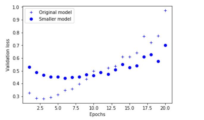

 

 

Add weight regularization

You may know the Occam's razor principle: if there are two explanations for a thing, the most likely correct explanation is the simplest one, that is, the one with fewer assumptions. This principle also applies to the models learned by neural networks: given some training data and a network architecture, many groups of weight values (i.e. many models) can interpret these data. Simple models are more difficult to over fit than complex models.

The simple model here refers to the model with less entropy of parameter value distribution (or the model with fewer parameters, such as the example in the previous section). Therefore, a common method to reduce over fitting is to force the model weight to take only a small value, so as to limit the complexity of the model, which makes the distribution of weight values more regular. This method is called weight regularization. Its implementation method is to add the cost related to the larger weight value to the network loss function. There are two forms of this cost.

• L1 regularization: the added cost is directly proportional to the absolute value of the weight coefficient [L1 norm of the weight].
• L2 regularization: the added cost is directly proportional to the square of the weight coefficient (L2 norm of the weight). L2 regularization of neural networks is also called weight decay. Don't be confused by different names. Weight attenuation is mathematically identical to L2 regularization.

In Keras, the method of adding weight regularization is to pass the weight regularizer instance to the layer as the keyword parameter. The following code will add L2 weight regularization to the film review classification network.

from keras import regularizers
​
l2_model = models.Sequential()
l2_model.add(layers.Dense(16, kernel_regularizer=regularizers.l2(0.001),
                          activation='relu', input_shape=(10000,)))
l2_model.add(layers.Dense(16, kernel_regularizer=regularizers.l2(0.001),
                          activation='relu'))
l2_model.add(layers.Dense(1, activation='sigmoid'))

l2_model.compile(optimizer='rmsprop',
                 loss='binary_crossentropy',
                 metrics=['acc'])

l2(0.001)   It means that each coefficient of the layer weight matrix will increase the total network loss   0.001 * weight_coefficient_value. Note that since this penalty item is only added during training, the training loss of this network will be much greater than the test loss.  

 

l2_model_hist = l2_model.fit(x_train, y_train,
                             epochs=20,
                             batch_size=512,
                             validation_data=(x_test, y_test))

l2_model_val_loss = l2_model_hist.history['val_loss']
​
plt.plot(epochs, original_val_loss, 'b+', label='Original model')
plt.plot(epochs, l2_model_val_loss, 'bo', label='L2-regularized model')
plt.xlabel('Epochs')
plt.ylabel('Validation loss')
plt.legend()
​
plt.show()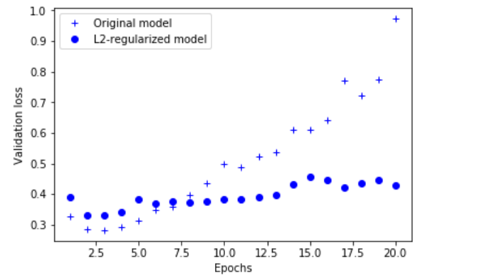

 

from keras import regularizers
​
# L1 regularization
regularizers.l1(0.001)
​
# L1 and L2 regularization at the same time
regularizers.l1_l2(l1=0.001, l2=0.001)

 

Add dropout regularization

Dropout is one of the most effective and commonly used regularization methods for neural networks. It was developed by Geoffrey Hinton of the University of Toronto and his students. Using dropout for a layer means that some output features of the layer are randomly discarded (set to 0) during training. Suppose that in the training process, the return value of a layer for a given input sample should be a vector   [0.2, 0.5, 1.3, 0.8, 1.1]. After using dropout, several random elements of this vector will become 0, such as   [0, 0.5,1.3, 0, 1.1]. The dropout rate is the proportion of features set to 0, usually in the range of 0.2 ~ 0.5. During the test, no units are discarded, and the output value of this layer needs to be reduced according to the dropout ratio, because at this time, more units are activated than during the training and need to be balanced.

Suppose there is a Numpy matrix containing the output of a layer   layer_output, whose shape is   (batch_size, features). During training, we randomly set some values in the matrix to 0.

dpt_model = models.Sequential()
dpt_model.add(layers.Dense(16, activation='relu', input_shape=(10000,)))
dpt_model.add(layers.Dropout(0.5))
dpt_model.add(layers.Dense(16, activation='relu'))
dpt_model.add(layers.Dropout(0.5))
dpt_model.add(layers.Dense(1, activation='sigmoid'))
​
dpt_model.compile(optimizer='rmsprop',
                  loss='binary_crossentropy',
                  metrics=['acc'])

dpt_model_hist = dpt_model.fit(x_train, y_train,
                               epochs=20,
                               batch_size=512,
                               validation_data=(x_test, y_test))

dpt_model_val_loss = dpt_model_hist.history['val_loss']
​
plt.plot(epochs, original_val_loss, 'b+', label='Original model')
plt.plot(epochs, dpt_model_val_loss, 'bo', label='Dropout-regularized model')
plt.xlabel('Epochs')
plt.ylabel('Validation loss')
plt.legend()
​
plt.show()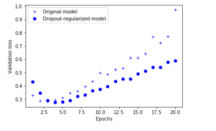

To sum up, common methods to prevent over fitting of neural networks include:

• Get more training data
• Reduce network capacity
• Add weight regularization
• Add dropout