Catalog
1. Decision Tree Model Data Classification
2. Decision tree pruning alleviates over-fitting problems
*Common decision tree algorithms are ID3, C4.5, and CART. The ID3 algorithm, proposed by Quinlan, an Australian computer scientist, in 1986, is one of the classic decision tree algorithms. The ID3 algorithm uses information gain to select when choosing attributes that divide nodes. Because the ID3 algorithm cannot handle non-discrete features, and because it does not take into account the sample size of each node, the ID3 algorithmThe C4.5 algorithm is a further improvement of the ID3 algorithm, which is capable of handling discontinuous features. When choosing attributes to divide nodes, the information gain rate is used to select them. Because the information gain rate takes into account the split information of nodes, it does not overfavor discrete features with a large number of values.The ID3 algorithm and the 44.5 algorithm are mainly used to solve classification problems, not regression problems, while the CART (Classification And Regression Tree) algorithm can handle both classification and regression problems. The CART algorithm uses Gini coefficients (Gini coefficients) to solve classification problems.The descent value selects the measure that divides the attributes of the nodes. When solving the regression problem, the descent value of variance of the target eigenvalue of the node data is used as the measure of the node classification.
The content of this article is to show the contents of the section on data classification of decision trees in the book "Python Machine Learning Algorithms and Warfare" (from the perspective of Bowen) - Sun Yulin, the other national books. Here is how to use the Sklearn Library in Python to complete the classification task of decision trees.

Book Cover
1. Decision Tree Model Data Classification
When building a decision data classification model, the pre-processed Titanic dataset is used, and the pre-processed data is sliced using the following methods:
import seaborn as sns
sns.set(font= "Kaiti",style="ticks",font_scale=1.4)
import numpy as np
import pandas as pd
import matplotlib.pyplot as plt
from sklearn.preprocessing import LabelEncoder
from sklearn.model_selection import  train_test_split
from sklearn.model_selection import GridSearchCV
from sklearn.tree import *
from sklearn.metrics import *
from io import StringIO
import graphviz
import pydotplus
# Targeted variable name for prediction
Target = ["Survived"]
## Define the name of the independent variable for the model
train_x = ["Pclass", "Name", "Sex", "Age", "SibSp", "Parch",
           "Fare","Embarked", "IsAlone"]
##Divide training set into training set and validation set
# Targeted variable name for prediction
Target = ["Survived"]
## Define the name of the independent variable for the model
train_x = ["Pclass", "Name", "Sex", "Age", "SibSp", "Parch",
           "Fare","Embarked", "IsAlone"]
##Divide training set into training set and validation set
X_train, X_val, y_train, y_val = train_test_split(
    train_pro[train_x], train_pro[Target],
    test_size = 0.25,random_state = 1)
print("X_train.shape :",X_train.shape)
print("X_val.shape :",X_val.shape)
print(X_train.head())
Out[9]:
X_train.shape : (668, 9)
X_val.shape : (223, 9)
     Pclass  Name  Sex   Age  SibSp  Parch     Fare  Embarked  IsAlone
35        1     2    1  42.0      1      0  52.0000         2        0
46        3     2    1  31.2      1      0  15.5000         1        0
453       1     2    1  49.0      1      0  89.1042         0        0
291       1     3    0  19.0      1      0  91.0792         0        0
748       1     2    1  19.0      1      0  53.1000         2        0
After partitioning the training set, 668 samples from the training set will be trained in the model, and the remaining samples will be used to verify the generalization ability of the model.
First, a decision tree model is built using the default parameters in the DecisionTreeClassifier() function, and the prediction accuracy on the training set and the verification set is calculated as follows:
## Set up a decision tree model with default parameters first
dtc1 = DecisionTreeClassifier(random_state=1)
## Training using training data
dtc1 = dtc1.fit(X_train, y_train)
## Output its prediction accuracy on training data and validation datasets
dtc1_lab = dtc1.predict(X_train)
dtc1_pre = dtc1.predict(X_val)
print("Accuracy on training datasets:",accuracy_score(y_train,dtc1_lab))
print("Verify accuracy on datasets:",accuracy_score(y_val,dtc1_pre))
Accuracy on training datasets: 0.9910179640718563
 Verify accuracy on datasets: 0.726457399103139
*From the output of the program, it can be found that the precision of the established model on the training dataset is 0.99, while that on the validation set is only 0.72, which is an obvious signal of model over-fitting. In order to visualize the situation of the fitted decision tree, the results can be visually analyzed and the structure diagram of the over-fitting decision shown in Figure 1 can be obtained using the following program.
## Visualize the resulting decision tree structure
dot_data = StringIO()
export_graphviz(dtc1, out_file=dot_data,
                feature_names=X_train.columns,
                filled=True, rounded=True,special_characters=True)
graph = pydotplus.graph_from_dot_data(dot_data.getvalue())
Image(graph.create_png())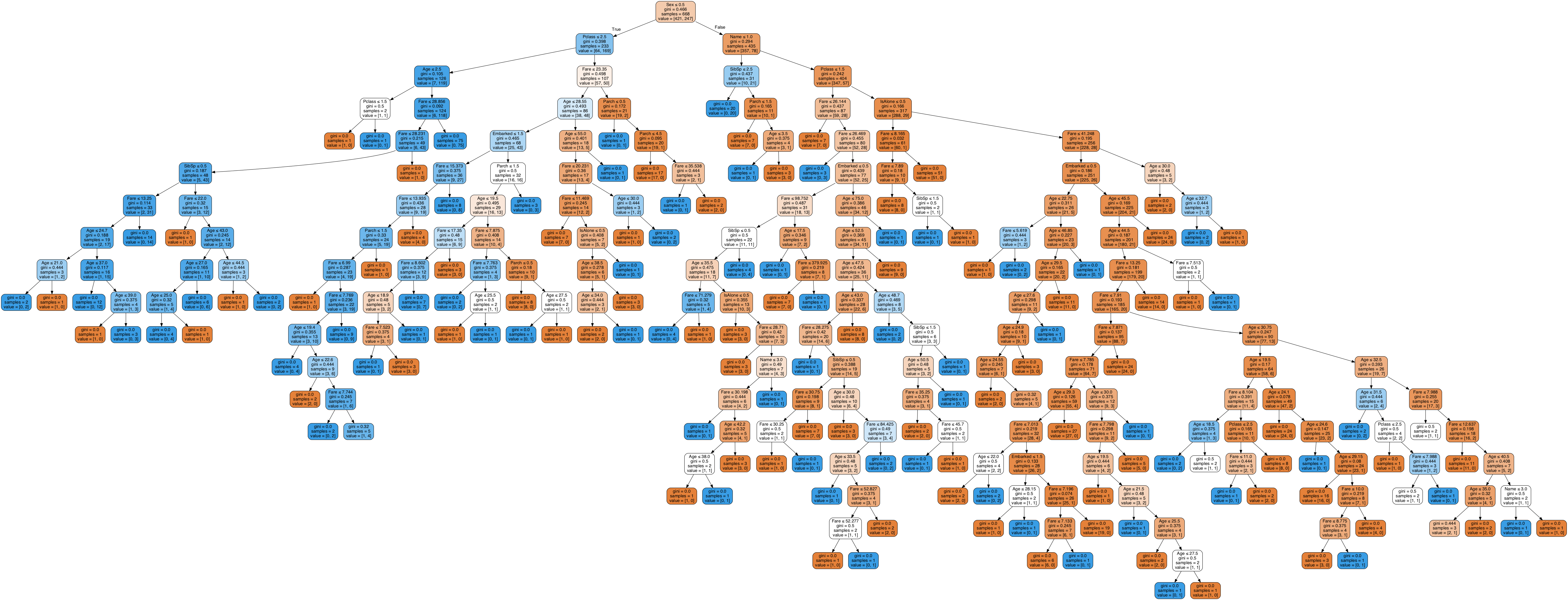
Figure 1: Fitted decision tree model
Looking at the model structure shown in Fig.1, we can see that the model is a very complex decision tree model, and the number of layers of the decision tree is far more than 10, which makes the rules obtained by using the decision tree very complex. The visualization of the model further proves that the obtained decision tree model has a serious over-fitting problem and needs to prune and simplify the model.
2. Decision tree pruning alleviates over-fitting problems
DecisionTreeClassifier() is used for pruning decision tree models.Two parameters in the function, max_depth and max_leaf_nodes, in which max_depth specifies the maximum depth of the decision tree and max_leaf_nodes specifies the maximum number of leaf nodes in the model. Here, two parameters in the model are searched using a parameter grid search, and the prediction accuracy on the validation set is quasi-measured to obtain a more appropriate combination of model parameters.The order is as follows:
## Finding appropriate decision tree model parameters using parameter grid search
depths = np.arange(3,20,1)
leafnodes = np.arange(10,30,2)
tree_depth = []
tree_leafnode = []
val_acc = []
for depth in depths:
    for leaf in leafnodes:
        dtc2 = DecisionTreeClassifier(max_depth=depth, ## Maximum Depth
                                      max_leaf_nodes=leaf,##Maximum number of leaf nodes
                                      min_samples_leaf=5,
min_samples_split=2,
                                      random_state=1)
        dtc2 = dtc2.fit(X_train,y_train)
        ## Calculate Prediction Accuracy on Test Set
        dtc2_pre = dtc2.predict(X_val)
        val_acc.append(accuracy_score(y_val,dtc2_pre))
        tree_depth.append(depth)
        tree_leafnode.append(leaf)
## Compose the results into a data table and output a good combination of parameters
DTCdf = pd.DataFrame(data = {"tree_depth":tree_depth,
                             "tree_leafnode":tree_leafnode,
                             "val_acc":val_acc})
## Sort by accuracy on validation set
print(DTCdf.sort_values("val_acc",ascending=False).head(15))

    tree_depth  tree_leafnode   val_acc
0            3             10  0.811659
1            3             12  0.811659
2            3             14  0.811659
3            3             16  0.811659
4            3             18  0.811659
5            3             20  0.811659
6            3             22  0.811659
7            3             24  0.811659
8            3             26  0.811659
9            3             28  0.811659
99          12             28  0.807175
98          12             26  0.807175
89          11             28  0.807175
88          11             26  0.807175
68           9             26  0.807175
From the output of the above program, it can be found that the effect of the number of leaf nodes on the Titanic data at the same tree depth is not significant. The following program trains a decision tree model with a more appropriate set of parameters, as shown below:
## Establishing a decision tree classifier with more appropriate parameters
dtc2 = DecisionTreeClassifier(max_depth=3, ## Maximum Depth
                              max_leaf_nodes=10, ## Maximum number of leaf nodes
                              min_samples_leaf=5,min_samples_split=2,
                              random_state=1)
dtc2 = dtc2.fit(X_train,y_train)
## Output its prediction accuracy on training data and validation datasets
dtc2_lab = dtc2.predict(X_train)
dtc2_pre = dtc2.predict(X_val)
print("Accuracy on training datasets:",accuracy_score(y_train,dtc2_lab))
print("Verify accuracy on datasets:",accuracy_score(y_val,dtc2_pre))
Accuracy on training datasets: 0.842814371257485
 Verify accuracy on datasets: 0.8116591928251121
By running the above program, you can see from the output results that the precision on the training set is 0.84 < 0.99 and on the validation set is 0.8116 > 0.72, which indicates that the over-fitting problem of the decision tree has been alleviated to some extent, and the model generalization ability obtained is stronger.
The following program can get the structure of the pruned decision tree model, and running the program can get the image shown in Figure 2.
## Visualizing the tree structure of a decision tree after pruning
dot_data = StringIO()
export_graphviz(dtc2, out_file=dot_data,
feature_names=X_train.columns,
filled=True, rounded=True,special_characters=True)
graph = pydotplus.graph_from_dot_data(dot_data.getvalue())
Image(graph.create_png())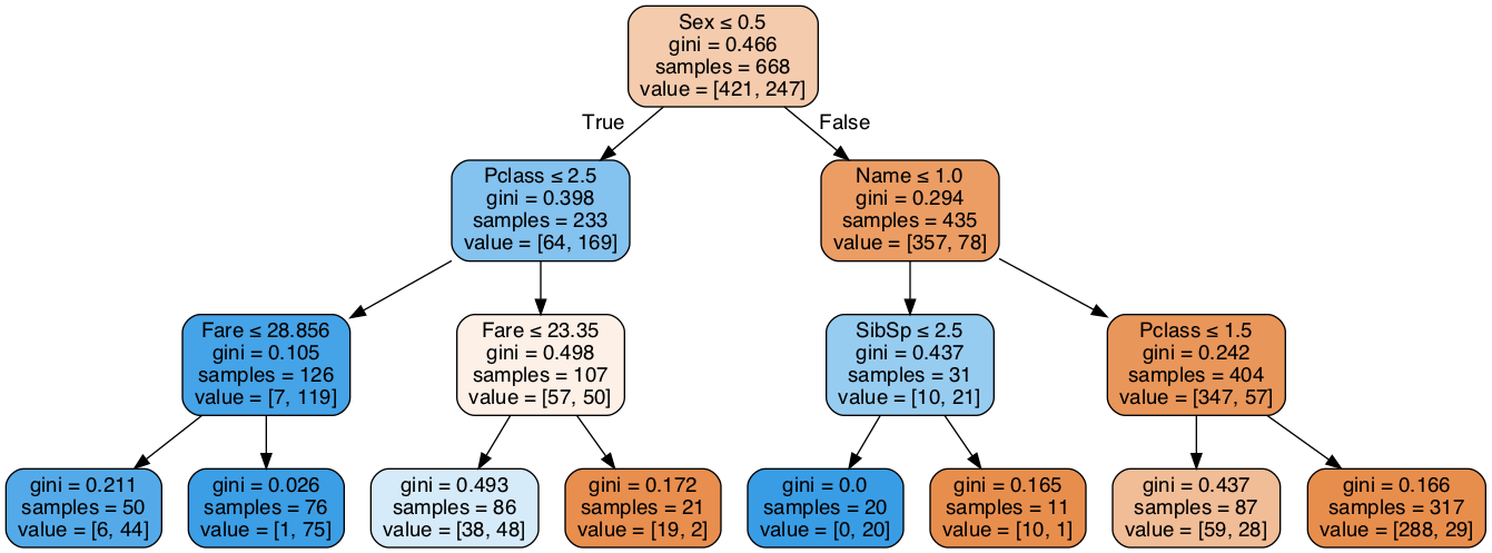 Figure 2. Decision tree model after pruning
From the decision tree model after pruning in Figure 2, it can be found that the model has been greatly simplified compared with the model without pruning. The root node is the Sex (gender) feature, that is, if Sex_Code<=0.5, go to the left branch to see the Pclass (ticket grade) feature, otherwise look at the right branch Name (salutation label, Mr., Ms.)The decision tree model after pruning is more intuitive and easier to analyze and interpret than the model without pruning.
The book can already be purchased in major online bookstores such as Jingdong and Dangdang (now 100 minus 50).
Welcome to our attention