search

1. Sequential search

• Through subscripts, we can access and search data items in order. This technology is called "sequential search"

def sequentialSearch(alist,item):
    pos = 0
    found = False

    while pos<len(alist) and not found:
        if alist[pos] == item:
            found = True
        else:
            pos = pos + 1

    return  found

testlist = [1, 2,32,8,17, 19, 42,13, 0]
print( sequentialSearch(testlist,3))
print ( sequentialSearch(testlist, 13))

# result 
"""
False
True
"""

• In the sequential search algorithm, in order to ensure that it is the general case discussed, it is necessary to assume that the data items in the list are not arranged in the order of values, but are randomly placed in each position in the list (in other words, the probability of data items appearing everywhere in the list is the same)
• Analysis of sequential search algorithm for unordered tables

If the data item is not in the list, you need to compare all the data items to know. The comparison times are n


If the data item is in the list, the number of times to compare is more complex
 Because the probability of data items appearing at each position in the list is the same; So on average, the number of comparisons is n/2；

Therefore, the algorithm complexity of sequential search is O(n)

• Sequential search of ordered table: it is almost the same as that of unordered table, but the ordered table can end in advance. For example, the search is 50, and the comparison is 54 (the data is in ascending order), indicating that the following data is greater than 50, there can be no 50, and you can exit in advance
• Sequential table sequential search code

def orderedSequentialSearch(alist, item):
    pos = 0
    found = False
    stop = False
    while pos < len(alist) and not found and not stop:
        if alist[pos] == item:
            found = True
        else:
            if alist[pos] > item:
                stop = True
            else:
                pos = pos+1
    return found

testlist = [0, 1, 2, 8, 13, 17, 19, 32, 42,]
print(orderedSequentialSearch(testlist, 3))
print(orderedSequentialSearch(testlist, 13))

• Analysis of sequential search algorithm for ordered table

If the data item is not in the list, the average number of comparisons is n/2


If the data item is in the list, the number of times to compare is more complex
 Because the probability of data items appearing at each position in the list is the same; So on average, the number of comparisons is n/2；

In fact, even in terms of legal complexity, it is still O(n)

Only when the data item does not exist, the search of the ordered table can save some comparison times, but does not change its order of magnitude

2. Binary search

• Compare from the middle of the list
  If the item in the middle of the list matches the search item, the search ends
  If not, there are two situations:
  • if the middle item of the list is larger than the search item, the search item may only appear in the first half
  • if the middle item of the list is smaller than the search item, the search item may only appear in the second half
  In any case, we will reduce the comparison range to half of the original: n/2
  Continue to use the above method to search, and each time the comparison range will be reduced by half
  This search method is binary search

• Binary search: Code

def binarySearch(alist, item):
    first = 0
    last = len(alist)-1
    found = False
    while first<=last and not found:
        midpoint = (first + last)//2
        if alist[midpoint] == item:  # Intermediate term comparison
            found = True
        else:
            if item < alist[midpoint]: # Narrow the contrast range
                last = midpoint-1
            else:
                first = midpoint+1
    return found

testlist = [0, 1, 2, 8, 13, 17, 19, 32, 42,]
print (binarySearch(testlist, 3))
print ( binarySearch(testlist, 13))

# result 
"""
False
True
"""

# Binary search algorithm actually embodies a typical strategy to solve the problem: divide and conquer
# The problem is divided into several smaller parts. The solution of the original problem is obtained by solving each small part of the problem and summarizing the results
# Obviously, recursive algorithm is a typical divide and conquer strategy algorithm, and dichotomy is also suitable for recursive algorithm

def binarySearch(alist, item):
    if len(alist) == 0:
        return False
    else:
        midpoint = len(alist)//2
        if alist [midpoint ]==item:
            return True
        else:
            if item<alist [midpoint] :
                return binarySearch( alist[ : midpoint], item)
            else:
                return binarySearch(alist [midpoint+1:], item)

testlist = [0, 1, 2, 8, 13, 17, 19, 32, 42,]
print (binarySearch(testlist, 3))
print ( binarySearch(testlist, 13))

# result 
"""
False
True
"""

• Analysis of binary search algorithm

Due to binary search, each comparison will reduce the comparison scope of the next step by half
 When the comparison times are enough, only one data item will remain in the comparison range
 Whether the data item matches the search item or not, the comparison will eventually end
n/2^i = 1
i = log2(n)
So the algorithm complexity of dichotomy search is O(log n)
Although we get the complexity of binary search according to the number of comparisons O(log n)
However, in addition to comparison, there is another factor to be noted in this algorithm:
binarySearch(alist[:midpoint],item)
This recursive call uses list slicing, and the complexity of the slicing operation is O(k)，This will slightly increase the time complexity of the whole algorithm;
Of course, we use slicing for better program readability. In fact, we can not slice,
Just pass in the start and end index values, so there will be no time overhead of slicing.

In addition, although binary search is superior to sequential search in time complexity
 But also consider the cost of sorting data items 
If multiple searches can be carried out after one sorting, the cost of sorting can be diluted
 However, if the data set changes frequently and the number of searches is relatively small, it may be more economical to directly use the unordered table and sequential search

Therefore, in the problem of algorithm selection, it is not enough to only look at the advantages and disadvantages of time complexity, but also consider the actual application

3. Hash

• Some basic concepts of hash

Previously, we used the knowledge about the arrangement relationship between data items in the data set to improve the search algorithm
 If the data items are arranged in order according to size, binary search can be used to reduce the complexity of the algorithm.


Now we further construct a new data structure, which can reduce the complexity of the search algorithm to O(1)，
This concept is called hashing Hashing"

If we can reduce the number of searches to the constant level, we must have more a priori knowledge of the location of the data item.


If we know in advance where the data item to be found should appear in the data set, we can go directly to that location to see if the data item exists

The hash algorithm maps the binary value of any length to a short fixed length binary value. This small binary value is called the hash value. The hash value is unique to a piece of data
 And extremely compact numerical representation. If you hash a plaintext and change even one letter of the paragraph, the subsequent hash will produce different values. To find
 Hashing two different inputs of the same value is computationally impossible, so the hash value of the data can check the integrity of the data. It is generally used for fast search and
 encryption algorithm 

Hash table( hash table，Also known as hash table) is a data set, in which the storage mode of data items is particularly conducive to rapid search and location in the future.

Each storage location in the hash table is called a slot( slot)，It can be used to save data items. Each slot has a unique name.

The function that implements the conversion from data item to storage slot name is called hash function( hash function)

The proportion of slots occupied by data items is called the "load factor" of the hash table

• Example (more in-depth understanding of hashes)

For example, a hash table containing 11 slots whose names are 0～ 10
 Before inserting a data item, the value of each slot is None，Indicates an empty slot
 The function that implements the conversion from data item to storage slot name is called hash function( hash function)
In the following example, the hash function takes a data item as a parameter and returns an integer value of 0～ 10，Represents the slot number (name) of the data item store
 In order to save the data items to the hash table, we design the first hash function
    Data items: 54, 26, 93, 17, 77, 31
 A common hash method is "remainder". Divide the data item by the size of the hash table, and the remainder obtained is used as the slot number.

In fact, the "remainder" method will appear in all hash functions in different forms

Because the slot number returned by the hash function must be within the Hash list size range, the Hash list size is generally summed
 In this example, our hash function is the simplest remainder: h(item)= item % 11
 According to hash function h(item)，After calculating the storage location for each data item, the data item can be stored in the corresponding slot

Item     HashValue
54          10
26          4
93          5
17          6
77          0   
31          9
 After the 6 data items in the example are inserted, they occupy 6 of the 11 slots in the hash table
 The proportion of slots occupied by data items is called the "load factor" of hash table, where the load factor is 6/11

After all the data items are saved to the hash table, the search is very simple
 To search whether a data item exists in the table, we only need to use the same hash function to calculate the search item and test the slot corresponding to the returned slot number
 Whether there are data items.Realized O(1)Time complexity search algorithm.

However, you may also see the problem with this scheme. This group of data happens to occupy different slots

If you want to save 44, h(44)=0，It is assigned to the same 0 as 77#In the groove, this situation is called "punching"
Outburst collision" ，We will discuss the solution to this problem later

• Perfect Hashing Function

❖ Given a set of data items, if a hash function can map each data item to a different slot, the hash function can be called "perfect hash function"     
❖ For a fixed set of data, we can always find a way to design a perfect hash function   
❖ However, if the data items change frequently, it is difficult to have a systematic method to design the corresponding perfect hash function     
❖ One way to get a perfect hash function is to expand the capacity of the hash table so that all possible data items can occupy different slots      
❖ However, this method is not practical when the range of possible data items is too large         
(If we want to save the mobile phone number (11 digits), the perfect hash function requires the hash table to have 10 billion slots! It will waste too much storage space)      
❖ Second, a good hash function needs to have the least feature conflict (approximately perfect), low computational difficulty (low overhead), and fully disperse data items (save space)

• More uses for perfect hash functions

❖ In addition to arranging the storage location of data items in the hash table, hash technology is also used in many fields of information processing
❖ Because the perfect hash function can generate different hash values for any different data, if the hash value is regarded as the "fingerprint" or "summary" of the data, this feature is widely used in data consistency verification
    Generating a fixed length "fingerprint" from arbitrary length data also requires uniqueness, which is mathematically impossible, but the ingenious design of "quasi perfection"
    Hash functions can do this in a practical sense

❖As a data fingerprint function for consistency verification, the following characteristics are required
    Compressibility: for any length of data, the length of "fingerprint" is fixed;
    Computability: it is easy to calculate the "fingerprint" from the original data; (it is impossible to calculate the original data from the fingerprint);
    Anti modification: small changes to the original data will cause great changes in the "fingerprint";
    Anti conflict: given the original data and "fingerprint", it is very difficult to find the data (forged) with the same fingerprint

• Python hash library hashlib

# Python's own hash function library of MD5 and SHA series: hashlib
# It includes six hash functions such as md5 / sha1 / sha224 / sha256 /sha384 / sha512

import hashlib
print(hashlib.md5("hello world!".encode("utf8")).hexdigest())
print(hashlib.md5("hello world".encode("utf8")).hexdigest())
print(hashlib.sha1("hello world!".encode("utf8")).hexdigest())

m = hashlib.md5()
m.update("hello world!".encode("utf8"))

print(m.hexdigest())



result
"""
fc3ff98e8c6a0d3087d515c0473f8677
5eb63bbbe01eeed093cb22bb8f5acdc3
430ce34d020724ed75a196dfc2ad67c77772d169
fc3ff98e8c6a0d3087d515c0473f8677
"""

• Perfect hash function for data consistency verification

❖Data file consistency judgment
❖Calculate the hash value for each file, and only compare the hash value to know whether the file content is the same;
❖Used for network file download integrity verification;
❖For file sharing system: the same files (especially movies) in the network disk can be stored without multiple times
❖Save password in encrypted form
❖Only the hash value of the password is saved. After the user enters the password, the hash value is calculated and compared;
❖It is not necessary to save the plaintext of the password to judge whether the user has entered the correct password.
(Calculating hash values from values is simple, but the reverse is not possible)

• Hash function design: folding method

❖ The basic steps of designing hash function by folding method are
    The data items are divided into several segments according to the number of digits,
    Add a few more numbers,
    Finally, the hash size is summed to obtain the hash value
❖ For example, for the phone number 62767255
    It can be divided into 4 segments (62, 76, 72, 55) in two digits
    Add (62)+76+72+55=265)
    The hash table includes 11 slots, which is 265%11=1
    therefore h(62767255)=1
❖ Sometimes the folding method also includes an interval inversion step
    For example, the interval number of (62, 76, 72, 55) is reversed to (62, 67, 72, 55)
    Re accumulation (62)+67+72+55=256)
    Remainder of 11 (256)%11=3)，therefore h'(62767255)=3
❖ Although interval inversion is not necessary in theory, this step does provide a fine-tuning means for the folding method to obtain the hash function, so as to better meet the hash characteristics

• Hash function design: square middle method

❖ Square middle method, first square the data item, then take the middle two digits of the square, and then remainder the size of the hash table
❖ For example, hash 44
    First 44*44=1936
    Then take the middle 93
    Remainder hash table size 11, 93%11=5

• Hash function design: non numeric terms

"""
❖ We can also hash non numeric data items and treat each character in the string as ASCII Code is enough
    as cat， ord('c')==99, ord('a')==96,ord('t')==116
❖ Then these integers are accumulated to sum up the size of the hash table
"""
def hash(astring,tablesize):
    sum = 0
    for pos in range(len(astring)):
        sum = sum + ord(astring[pos])

    return sum%tablesize

# The ord function can convert characters into ASCII code you need
# Of course, such a hash function returns the same hash value for all out of order words
# To prevent this, you can multiply the position of the string by the ord value as a weighting factor

• Hash function design

❖ We can also design more hash function methods, but a basic starting point to adhere to is that hash function can not become the computational burden of stored procedures and search procedures
❖ If the hash function design is too complex, it will cost a lot of computing resources to calculate the slot number,Lost the meaning of the hash itself
    It may be better to simply perform sequential search or binary search

• Conflict resolution

❖ If two data items are hashed to the same slot, a systematic method is needed to save the second data item in the hash table. This process is called "conflict resolution"
❖ As mentioned earlier, if the hash function is perfect, there will be no hash conflict, but the perfect hash function is often unrealistic
❖ Resolving hash conflicts has become a very important part of hash methods.
❖ One way to solve hash is to find an open empty slot for conflicting data items
    The simplest is to scan back from the conflicting slot until an empty slot is encountered
    If not found at the end of the hash table, scan from the head
❖ This technique for finding empty slots is called "open addressing" open addressing"
❖The backward slot by slot search method is "linear detection" in open addressing technology linear probing"

• Conflict resolution: Linear Probing
  [external chain picture transfer failed. The source station may have anti-theft chain mechanism. It is recommended to save the picture and upload it directly (img-mzgnuna9-1634894171242)( https://note.youdao.com/yws/res/c/WEBRESOURCE25547ea06df98ac432fd25d7be0d232c )]

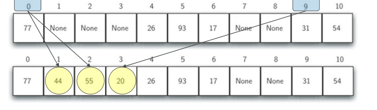
We insert 44, 55 and 20 into the hash table one by one
    h(44)=0，But found 0#Slot is occupied by 77. Find the first empty slot 1 backward#, save
    h(55)=0，Same 0#The slot has been occupied. Find the first empty slot 2 backward#, save
    h(20)=9，Discovery 9#The slot has been occupied by 31. Go back and find 3 from the beginning#Slot save
    
If the linear detection method is used to solve the hash conflict, the hash search also follows the same rules
    If the search term is not found in the hash position, you must search backward in order
    Until the search term is found or an empty slot is encountered (search fails).

• Conflict resolution: improvement of linear detection

❖ One disadvantage of linear detection method is aggregation( clustering)Trend of
❖ That is, if there are many conflicting data items in the same slot, these data items will gather near the slot
❖ So as to chain affect the insertion of other data items
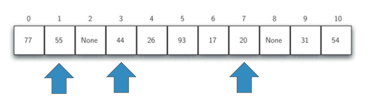
❖ One way to avoid aggregation is to expand linear detection from one by one to jump detection
    The following figure is“ +3" Probe inserts 44, 55, 20

• Conflict resolution: rehashing

❖ The process of re finding empty slots can be done with a more general "re hashing" rehashing" To summarize
    newhashvalue = rehash(oldhashvalue)
    For linear detection, rehash(pos)= (pos+ 1)%sizeoftable
    " +3" The hopping detection is: rehash(pos)=(pos+ 3)% sizeoftable
    The general hashing formula for skip detection is: rehash(pos)=(pos+skip)% sizeoftable

❖ In jump detection, it should be noted that skip The value of cannot be divided by the hash table size, otherwise a cycle will occur, resulting in many empty slots that can never be detected
    One trick is to set the size of the hash table to prime, as in example 11
    
❖ You can also change linear detection to "secondary detection" quadratic probing"
❖ No longer fixed skip But gradually increase skip Values, such as 1, 3, 5, 7, 9
❖ In this way, the slot number will be the original hash value, increasing by square: h, h+1, h+4, h+9, h+16...

• Conflict resolution: Data Necklace Chaining

❖In addition to the open addressing technology of finding empty slots, another solution to hash conflict is to expand the slot containing a single data item to accommodate a collection of data items (or a reference to a data Necklace table)
❖In this way, each slot in the hash table can accommodate multiple data items. If there is a hash conflict, you only need to simply add the data items to the data item collection.
❖When searching for data items, you need to search the entire set in the same slot. Of course, with the increase of hash conflict, the search time for data items will increase accordingly.

Mapping abstract data types and Python implementation

• Abstract data type mapping: ADT Map

❖ Python One of the most useful data types "dictionary"
❖ A dictionary is a kind of dictionary that can be saved key-data Data type of key value pair
    Where key key Can be used to query associated data values data
❖ This method of key value association is called mapping Map"
❖ ADT Map The structure of is a key-Unordered collection of values associated
    Keys are unique
    A data value can be uniquely determined by a key


realization ADT Map
❖ The advantage of using a dictionary is that given a key key，The associated data values can be obtained quickly data
❖ In order to achieve the goal of fast search, it is necessary to support efficient search ADT realization
    You can use list data structure plus sequential search or binary search. Of course, it is more appropriate to use the aforementioned hash table to achieve the fastest search O(1)Performance of

• Operations defined by ADT Map

Map(): Create an empty mapping and return the empty mapping object;
put(key, val): take key‐val If the association pair is added to the mapping key Already exists, will val Replace the old association value;
get(key): given key，Returns the associated data value. If it does not exist, it returns None；
del: adopt del map[key]Delete as a statement key‐val relation;
len(): Return to mapping key‐val Number of associations;
in: adopt key in map Statement form, return key Whether it exists in the association, Boolean

• Implementation example of ADT Map

#We use a HashTable class to implement ADT Map, which contains two lists as members
#    One of the slot lists is used to save the key
#    Another parallel data list is used to hold data items
# After the location of a key is found in the slot list, the data items corresponding to the same location in the data list are associated data

class HashTable:
    def __init__ (self):
        self.size = 11
        self.slots = [None]*self.size
        self.data = [None]*self.size

    def hashfunction(self, key):
        return key% self.size
    def rehash( self, oldhash):
        return (oldhash+ 1)% self.size
    def put(self,key,data):
        hashvalue = self.hashfunction(key)

        if self.slots [hashvalue] == None:
            self.slots[hashvalue] = key
            self.data [hashvalue] = data
        else:
            if self.slots [hashvalue] == key:
                self.data[hashvalue] = data #replace
            else:
                nextslot = self.rehash(hashvalue)

                while self.slots[nextslot] != None and self.slots [nextslot] != key:
                    nextslot = self.rehash(nextslot)
                if self.slots [nextslot] == None:
                    self . slots[nextslot]=key
                    self . data [nextslot]=data
                else:
                    self.data[nextslot] = data #replace

    def get(self,key):
        startslot = self.hashfunction(key)  # Mark the hash value as the starting point of the search
        data = None
        stop = False
        found = False
        position = startslot
        while self.slots[position] != None and not found and not stop:
            # Find the key until the slot is empty or back to the starting point
            if self.slots[position] == key:
                found = True
                data = self . data[position]
            else:
                position=self.rehash( position) # key not found, hash and continue to find
            if position == startslot:  # Back to the starting point, stop
                stop = True
        return data

    # [] access through special methods
    def __getitem__(self, key):
        return self.get(key)
    def __setitem__(self, key, data):
        self.put(key, data)


H=HashTable()
H[54]="cat"
H[26]= "dog"
H[93]="lion"
H[17]="tiger"
H[77]="bird"
H[31]="cow"
H[44]="goat"
H[55]="pig"
H[ 20]= "chicken"
print(H.slots)
print(H.data)
print(H[20])
print(H[17])
H[20]= 'duck'
print(H[20])
print(H[99])

# result
"""
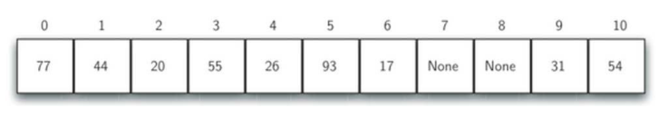
[77, 44, 55, 20, 26, 93, 17, None, None, 31, 54]
['bird', 'goat', 'pig', 'chicken', 'dog', 'lion', 'tiger', None, None, 'cow', 'cat']
chicken
tiger
duck
None
"""

• Hash algorithm analysis

❖ In the best case, hashing can provide O(1)Search performance of constant time complexity
    Due to the existence of hash conflict, the number of search comparisons is not so simple
❖ The most important information for evaluating hash conflicts is the load factorλ，
    In general:
    IfλSmaller, the probability of hash collision is small, and data items are usually saved in the hash slot to which they belong
    IfλLarger means that the hash table is filled with more and more conflicts, and the conflict resolution is more complex, so more comparisons are needed to find empty slots; if a data chain is used, it means that there are more data items on each chain
❖ If the open addressing method of linear detection is used to solve the conflict(λAt 0~1 Between)
    For successful searches, the average number of comparisons required is: 0.5*(1 + 1/(1-λ))  Unsuccessful search, average comparison times: 0.5*(1 + 1/(1-λ)^2)
❖ If the data link is used to solve the conflict(λ(can be greater than 1)
    The average number of comparisons required for a successful search is: 1 + λ/2
    For unsuccessful searches, the average comparison times are: λ

sort

1. Bubble Sort

# code
def bubbleSort(alist):

    for passnum in range(len(alist)-1,0,-1):
        for i in range(passnum):
            if alist[i]>alist[i+1]:
                temp = alist[i]
                alist[i] = alist[i+1]
                alist[i+1] = temp

alist = [54,26,93,17,77,31,44,55,20]
bubbleSort(alist)
print(alist)

# result
# [17, 20, 26, 31, 44, 54, 55, 77, 93]

# Bubble sorting: algorithm analysis
# The comparison times are the accumulation of 1 ~ n-1: 1/2 * n * (n-1)
# The time complexity of the comparison is O(n^2)

"""
❖ The time complexity is also related to the number of exchanges O(n2^)，Usually, each exchange includes 3 assignments
❖ The best case is that the list is ordered before sorting, and the number of exchanges is 0
❖ The worst case is that each comparison must be exchanged, and the number of exchanges is equal to the number of comparisons
❖ The average is half the worst
❖ Bubble sorting is usually used as a sorting algorithm with poor time efficiency as a benchmark for other algorithms.
❖ Its efficiency is mainly poor. Before finding its final location, each data item must be compared and exchanged many times, and most of the operations are invalid.
❖ But one advantage is that there is no additional storage overhead.
"""

# Performance improvement

"""
❖ In addition, by monitoring whether each comparison has been exchanged, it can determine whether the sorting is completed in advance
❖ This is what most other sorting algorithms cannot do
❖ If there is no exchange in a comparison, the list has been arranged, and the algorithm can be ended in advance"
"""
def shortBubbleSort(alist):
    exchanges = True
    passnum = len(alist)-1
    while passnum > 0 and exchanges:
        exchanges = False
        for i in range(passnum):
            if alist[i]>alist[i+1]:
                exchanges = True
                temp = alist[i]
                alist[i] = alist[i+1]
                alist[i+1] = temp
        passnum = passnum - 1
        
alist=[20,30,40,90,50, 60,70, 80, 100,110]
shortBubbleSort(alist)
print(alist)

# result
# [20, 30, 40, 50, 60, 70, 80, 90, 100, 110]

2. Select Sorting

"""
❖ Selective sorting improves bubble sorting, retains its basic multi pass comparison idea, and makes the current maximum item in place in each pass.
❖ However, sorting is selected to reduce the exchange. Compared with bubbling sorting, multiple exchanges are carried out, and only one exchange is carried out in each trip. The location of the largest item is recorded, and finally exchanged with the last item of this trip
❖ The time complexity of selective sorting is slightly better than bubble sorting
    The number of comparisons remains the same, or O(n2)
    The number of exchanges is reduced to O(n)
"""
def selectionSort(alist):
    for fillslot in range(len(alist)-1,0,-1):
        positionOfMax=0
        for location in range(1, fillslot+1):
            if alist[location]>alist[positionOfMax]:
                positionOfMax = location

        temp = alist[fillslot]
        alist[fillslot] = alist[positionOfMax]
        alist[positionOfMax] = temp

alist = [54,26,93,17,77,31,44,55,20]
selectionSort(alist)
print(alist)

# result
# [17, 20, 26, 31, 44, 54, 55, 77, 93]

3. Insertion Sort

"""
❖ In the first trip, the sub list only contains the first data item. Insert the second data item into the appropriate position of the sub list as a "new item", so that the sorted sub list contains two data items
❖ For the second time, continue to compare the third data item with the first two data items, move the data item larger than itself, and make space for adding to the sub list
❖ after n-1 Through comparison and insertion, the sub list is extended to the whole table, and the sorting is completed

❖ The comparison of insertion sort is mainly used to find the insertion position of "new item"
❖ The worst case is that each trip is compared with all items in the sub list. The total comparison times are the same as the bubble sort, and the order of magnitude is still the same O(n2)
❖ In the best case, when the list has been arranged, only one comparison is required for each trip, and the total number is O(n)
"""
def insertionSort(alist):
    for index in range(1,len(alist)):

        currentvalue = alist[index] #New item / insert item
        position = index

        while position>0 and alist[position-1]>currentvalue:
            alist[position]=alist[position-1]
            position = position-1    # Comparison and movement

        alist[position]=currentvalue # Insert new item


alist = [54,26,93,17,77,31,44,55,20]
insertionSort(alist)
print(alist)

# result
# [17, 20, 26, 31, 44, 54, 55, 77, 93]

4. Shell Sort

• We note that the comparison times of insertion sorting are O(n) in the best case. This happens when the list is already ordered. In fact, the closer the list is to order, the fewer the comparison times of insertion sorting

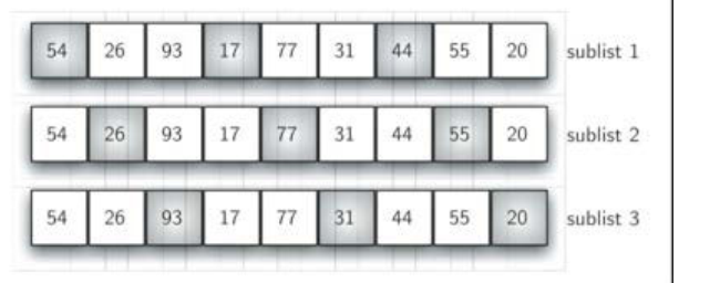
• Starting from this situation, Schell sort takes insertion sort as the basis, divides the unordered table into sub lists at an interval, and each sub list performs insertion sort
  

• As the number of sub lists decreases, the whole of the unordered table becomes closer and closer to order, so as to reduce the comparison times of the overall sorting

• For the sub list with an interval of 3, the overall situation of the sub list after being inserted and sorted is closer to order
  

• The last one is the standard insertion sort, but because the list has been processed to near order in the previous several times, this one only needs a few moves to complete

• The interval of sub list generally starts from n/2, and each trip is doubled: n/4, n/8... Until 1

def shellSort(alist):
    sublistcount = len(alist)//2 # interval setting
    while sublistcount > 0:

        for startposition in range(sublistcount): # Sub list sorting
            gapInsertionSort(alist , startposition, sublistcount)

        print("After increments of size" , sublistcount ,"The list is",alist)
        sublistcount = sublistcount // 2 # interval reduction

def gapInsertionSort (alist,start,gap):
    for i in range(start+gap,len(alist),gap):

        currentvalue = alist[i]
        position = i

        while position>=gap and alist [position-gap]>currentvalue:
            alist[position]=alist [position-gap]
            position = position-gap

        alist[position]=currentvalue

alist = [54,26,93,17,77,31,44,55,20]
shellSort(alist)

# result
"""
After increments of size 4 The list is [20, 26, 44, 17, 54, 31, 93, 55, 77]
After increments of size 2 The list is [20, 17, 44, 26, 54, 31, 77, 55, 93]
After increments of size 1 The list is [17, 20, 26, 31, 44, 54, 55, 77, 93]
"""

• Roughly speaking, Schell sort is based on insertion sort and may not be better than insertion sort
• However, because each trip brings the list closer to order, this process will reduce a lot of "invalid" comparisons originally required
  The detailed analysis of Schell sort is more complex, which is roughly between O(n) and O(n2)
• If the interval is kept at 2k-1(1, 3, 5, 7, 15, 31, etc.), the time complexity of Schell sorting is about O (n3/2)

4. Merge Sort

• Application of divide and conquer strategy in sorting
• Merge sort is a recursive algorithm. The idea is to continuously split the data table into two halves and merge and sort the two halves respectively
  The basic end condition of recursion is that the data table has only one data item, which is naturally in good order;
  Reduce the scale: split the data table into two equal halves and reduce the scale to one-half of the original;
  Call itself: sort the two halves separately, and then sort the two halves separately

def mergeSort(alist):
    if len(alist)>1:# Basic end condition
        mid = len(alist)//2
        lefthalf = alist[ :mid]
        righthalf = alist[mid:]

        mergeSort(lefthalf) # Recursive call
        mergeSort(righthalf)

        i=j=k=0
        while i<len(lefthalf) and j<len(righthalf):#Zipper interleaving brings the left and right halves from small to large into the result list
            if lefthalf[i]<righthalf[j]:
                alist[k]=lefthalf[i]
                i=i+1
            else:
                alist[k]=righthalf[j]
                j=j+1
            k=k+1

        while i<len(lefthalf):#Merge left half remainder
            alist[k]=lefthalf[i]
            i=i+1
            k=k+1
        while j<len(righthalf):#Merge the remaining items in the right half
            alist[k]=righthalf[j]
            j=j+1
            k=k+1


alist = [54,26,93,17,77,31,44,55,20]
mergeSort(alist)
print(alist)


# result
# [17, 20, 26, 31, 44, 54, 55, 77, 93]

# Another merge sort code
def merge_sort(lst):
    #Recursive end condition
    if len(lst) <= 1:
        return lst

    #Decompose the problem and call recursively
    middle = len(lst) // 2
    left = merge_sort(lst[:middle]) #Order the left half
    right = merge_sort(lst[middle:]) # Order the right half

    #Merge the left and right halves to complete the sorting
    merged = []
    while left and right :
        if left[0] <= right[0]:
            merged. append(left.pop(0))
        else:
            merged. append(right . pop(0))
    merged.extend(right if right else left)
    return merged



alist = [54,26,93,17,77,31,44,55,20]
print(merge_sort(alist))

# result
# [17, 20, 26, 31, 44, 54, 55, 77, 93]

• Merge sort: algorithm analysis

❖ The merging sort is divided into two processes: splitting and merging
❖ The splitting process, based on the analysis results in binary search, is logarithmic complexity, and the time complexity is O(log n)
❖ In the merging process, all data items will be compared and placed once relative to each part of the split, so it is a linear complexity and its time complexity is O(n)
    Considering comprehensively, each split part is carried out once O(n)The total time complexity of data item merging is O(nlog n)

❖ Finally, we note that the two slicing operations can be cancelled for the sake of accuracy of time complexity analysis,
   It's OK to pass the start and end points of the two split parts instead, but the readability of the algorithm is slightly sacrificed.
❖ We note that the merge sort algorithm uses an additional 1 times the storage space for merging ,This feature should be taken into account when sorting large data sets

5. Quick Sort

• The idea of quick sort is to divide the data table into two halves according to a "median" data item: less than half of the median and more than half of the median, and then quickly sort each part (recursion)
  If you want the two halves to have an equal number of data items, you should find the "median" of the data table
  But finding the median needs to calculate the cost! If you want to have no cost, you can only find a number at will as the "median"
  For example, the first number.
• Recursive algorithm for quick sorting "recursive three elements"

❖ Basic end condition: the data table has only one data item, which is naturally in good order
❖ Downsizing: divide the data sheet into two halves according to the "median", preferably two halves of the same size
❖ Call itself: sort the two halves separately
  (Sort basic operation (during splitting)

• code

"""
❖ The goal of splitting the data table: find the position of the "median"
❖ Means of splitting data tables
    Set left and right markers( left/rightmark)
    The left marker moves to the right and the right marker moves to the left
        • The left marker moves all the way to the right, and stops when it encounters something larger than the median value
        • The right mark moves to the left and stops when it is smaller than the median value
        • Then exchange the data items indicated by the left and right marks
    Continue moving until the left marker moves to the right of the right marker, and stop moving
    At this time, the position indicated by the right mark is the position where the "median" should be
    Swap the median with this position
    After division, the left half is smaller than the median, and the right half is larger than the median
"""
def quickSort(alist):
    quickSortHelper(alist,0,len(alist)-1)

def quickSortHelper(alist, first,last):
    if first<last:   #Basic end condition

        splitpoint = partition(alist, first,last)# division

        quickSortHelper(alist , first , splitpoint-1)#Recursive call
        quickSortHelper( alist , splitpoint+1,last)

def partition(alist, first, last):
    pivotvalue = alist[first] #Select median“

    leftmark = first + 1 #Left and right initial values
    rightmark = last

    done = False
    while not done:
        while leftmark <= rightmark and alist[leftmark] <= pivotvalue:
            leftmark = leftmark + 1 #Move left marker to the right

        while alist[rightmark] >= pivotvalue and rightmark >= leftmark:
            rightmark = rightmark - 1 #Move right marker left

        if rightmark < leftmark: #The movement ends when the two marks are wrong
            done = True
        else: #Left and right standard value exchange
            temp = alist[leftmark]
            alist[leftmark] = alist[rightmark]
            alist[rightmark] = temp

    temp = alist[first] #Median in place
    alist[first] = alist[rightmark]
    alist[rightmark] = temp

    return rightmark # The median point is also the splitting point


alist = [54, 26, 93, 17, 77, 31, 44, 55, 20]
quickSort(alist)
print(alist)

# result
# [17, 20, 26, 31, 44, 54, 55, 77, 93]

• Quick sort: algorithm analysis

❖ The quick sort process is divided into two parts: splitting and moving
    If splitting always divides the data table into two equal parts, it is O(logn)Complexity of;
    And mobile needs to compare each item with the median, or O(n)
❖ Taken together O(nlog n)；
❖ Moreover, no additional storage space is required during the operation of the algorithm.

❖ However, if not so lucky, the split point of the median is too far away from the middle, resulting in an imbalance between the left and right parts
❖ In extreme cases, there is always no data in some parts, so the time complexity degrades to O(n2)
    Plus the overhead of recursive calls (worse than bubble sorting)

❖ The selection method of the lower median can be appropriately improved to make the median more representative
    For example, "three-point sampling", select the median value from the head, tail and middle of the data table
    There will be additional computational overhead, and extreme cases cannot be ruled out

Algorithm complexity summary

• The time complexity of sequential search on unordered or ordered tables is O(n)

• The worst complexity of binary search on ordered table is O(log n)

• Hash table can realize constant time search

• Perfect hash function is widely used as data consistency verification

• Bubbling, selection and insertion sorting are O(n2) algorithms

• Schell sort is improved on the basis of insertion sort. The method of sorting incremental sub tables is adopted, and its time complexity can be between O(n) and O(n2)

• The time complexity of merging sorting is O(nlog n), but the merging process requires additional storage space

• The best time complexity of quick sorting is O(nlog n), and no additional storage space is required. However, if the splitting point deviates from the center of the list, it will degenerate to O(n2) in the worst case