Catalog
In the previous section [python data analysis practice] box office data analysis (I) data collection The box office data from 2011 to now has been obtained and saved in mysql.
This paper will explain how to extract the data in mysql and make it dynamic visualization in practice.
Figure 1 trend of monthly ticket house every year
The first picture, we want to look at the monthly box office trend, there is no doubt to make a line chart, nearly 10 years of box office data on one picture.
Data extraction:
The box office data collected is calculated by day, and we only see the normal release and click Show, other shows such as remake are not included in this statistics.
Therefore, we first filter the data releaseInfo field in mysql, and then group and aggregate according to the release year and month to get the monthly box office data within 10 years.
After fetching the data with sql, put the data of different years into the list respectively. The original data is str in the unit of "ten thousand". Here we convert it to float in the unit of "hundred million".
Construct image:
The x-axis data is the year.
Then add the box office data of different years to the y-axis.
Finally, configure the image properties.
config = {...}    # db configuration omitted
conn = pymysql.connect(**config)
cursor = conn.cursor()
sql = '''
        select  substr(`date`,1,4) year,
                substr(`date`,5,2) month,
                round(sum(`boxInfo`),2) monthbox
        from movies_data
        where (substr(`releaseInfo`,1,2) = 'Release' or `releaseInfo`='Point projection' )
        group by year,month order by year,month
      '''
cursor.execute(sql)
data = cursor.fetchall()
x_data = list(set([int(i[1]) for i in data]))
x_data.sort()
x_data = list(map(str, x_data))
y_data1 = [round(int(i[2]) / 10000, 2) for i in data if i[0] == '2011']
y_data2 = [round(int(i[2]) / 10000, 2) for i in data if i[0] == '2012']
y_data3 = [round(int(i[2]) / 10000, 2) for i in data if i[0] == '2013']
y_data4 = [round(int(i[2]) / 10000, 2) for i in data if i[0] == '2014']
y_data5 = [round(int(i[2]) / 10000, 2) for i in data if i[0] == '2015']
y_data6 = [round(int(i[2]) / 10000, 2) for i in data if i[0] == '2016']
y_data7 = [round(int(i[2]) / 10000, 2) for i in data if i[0] == '2017']
y_data8 = [round(int(i[2]) / 10000, 2) for i in data if i[0] == '2018']
y_data9 = [round(int(i[2]) / 10000, 2) for i in data if i[0] == '2019']
cursor.close()
conn.close()


def line_base() -> Line:
    c = (
        Line(init_opts=opts.InitOpts(height="600px", width="1300px"))
            .add_xaxis(x_data)
            .add_yaxis("2011", y_data1)
            .add_yaxis("2012", y_data2)
            .add_yaxis("2013", y_data3)
            .add_yaxis("2014", y_data4)
            .add_yaxis("2015", y_data5)
            .add_yaxis("2016", y_data6)
            .add_yaxis("2017", y_data7)
            .add_yaxis("2018", y_data8)
            .add_yaxis("2019", y_data9)
            .set_global_opts(title_opts=opts.TitleOpts(title="Monthly box office trend"),
                             legend_opts=opts.LegendOpts(
                                 type_="scroll", pos_top="55%", pos_left="95%", orient="vertical"),
                             xaxis_opts=opts.AxisOpts(
                                 axistick_opts=opts.AxisTickOpts(is_align_with_label=True), boundary_gap=False, ),)
            .set_series_opts(label_opts=opts.LabelOpts(is_show=False),  # Do not display dimensions on columns (numeric)
                             markline_opts=opts.MarkLineOpts(
                                 data=[opts.MarkLineItem(type_="max", name="Maximum value"), ]), )
            .extend_axis(yaxis=opts.AxisOpts(name="box office(Billion yuan)", position='left'),  # Set the display format of y-axis label, data + person
                              xaxis=opts.AxisOpts(name="Month"))
    )

    return c


line_base().render("v1.html")
As can be seen from this figure:
1. The total number of box office has gradually increased in the past 10 years (this is nonsense, of course)
2. The monthly box office fluctuation of 11-13 years is very small, and there is almost no obvious peak schedule. The most obvious peak schedule in the recent two years is the Spring Festival, summer vacation and the 11th.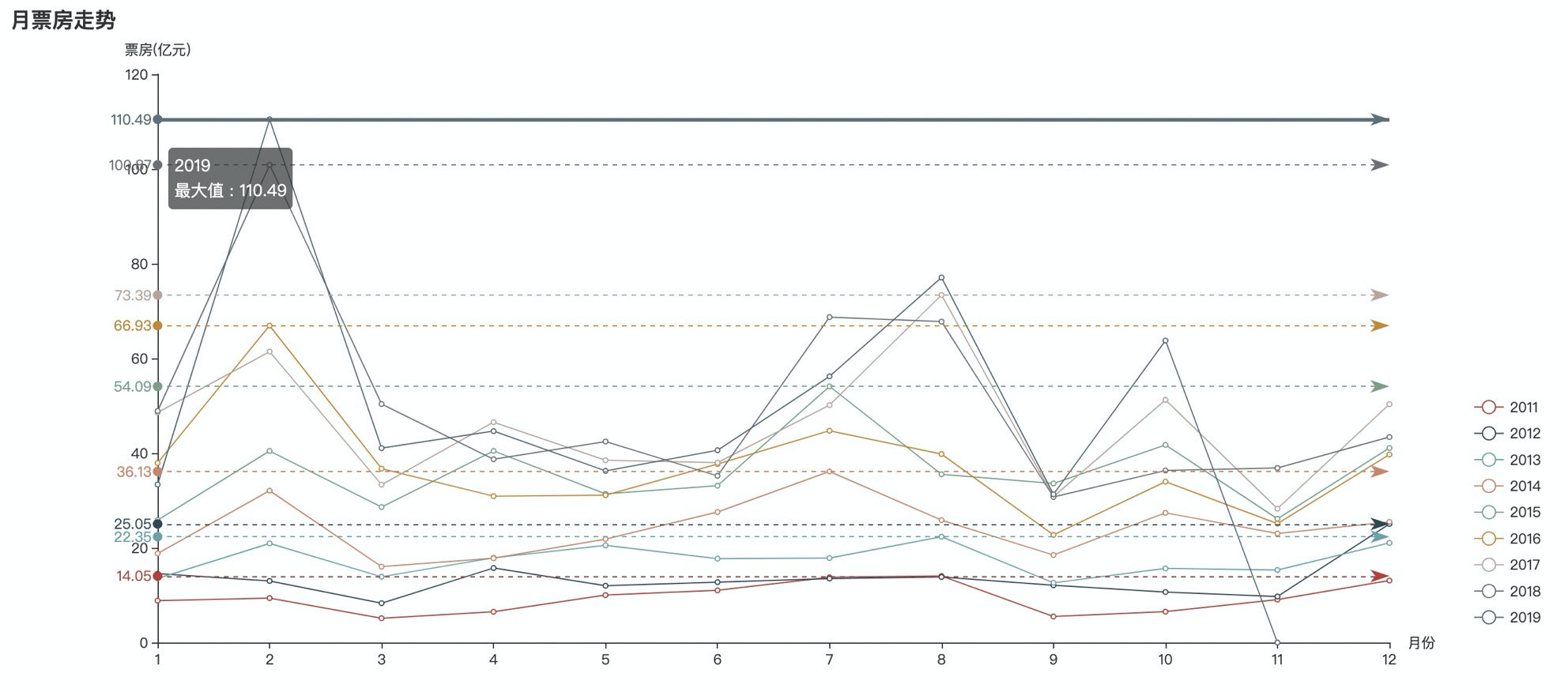
Figure 2 total box office value, total number of films released and number of audience
In the second picture, we want to see the change of box office, the number of films released and the number of people watching movies year by year.
Data extraction:
First, filter the releaseInfo data for normal release and premiere.
Then group by year, which is the first four digits of the date field.
- sum the box office fields of the day to get the total box office of the year;
- De duplicate the movieId field and find the number of times of occurrence, which is the total number of films released.
- The average number of people * row times is the number of people watching movies on that day, and then sum up the number of people watching movies every year.
Construct image:
Because the x-axis of the three types of data is the year, it can be displayed on a map. In order to observe more intuitively, one of the data is made into a column chart, and the other two are made into a line chart.
- 1. First, construct a line chart, add box office and movie quantity as y-axis data, and year as x-axis data.
- 2. Because the value range of box office and the number of films released is basically the same after unit conversion, a y-axis can be shared, and a separate y-axis is needed for the audience.
So we need to add a new y-axis, and specify the y-axis index of the three data respectively, that is, the default Y-axis index for box office and number of films released is 0, and the y-axis Index added after the number of people watching the movie is 1. - 3. Reconstruct the histogram. The y-axis data is the number of people watching the movie, the x-axis data is still the year, and the y-axis index is 1.
- 4. Finally, overlap the histogram and line graph, and simply adjust the image position.
config = {...}    # db configuration omitted
conn = pymysql.connect(**config)
cursor = conn.cursor()
sql2 = '''select substr(date,1,4),
                 round(sum(boxInfo)/10000,2),
                 count(DISTINCT movieId),
                 round(sum(avgShowView*showInfo)/100000000,2)
            from movies_data
            where (substr(`releaseInfo`,1,2) = 'Release' or `releaseInfo`='Point projection' )
            GROUP by substr(date,1,4)'''
cursor.execute(sql2)
data2 = cursor.fetchall()
x_data2 = [i[0] for i in data2]
y_data2_1 = [i[1] for i in data2]
y_data2_2 = [i[2] for i in data2]
y_data2_3 = [i[3] for i in data2]
cursor.close()
conn.close()


def bar_base() -> Line:
    c = (
        Line()
            .add_xaxis(x_data2)
            .add_yaxis("Total box office", y_data2_1, yaxis_index=0)
            .add_yaxis("Total number of films released", y_data2_2, color='LimeGreen', yaxis_index=0, )
            .set_global_opts(title_opts=opts.TitleOpts(title="Total annual box office value, total number of films released and total number of people watching films"),
                             legend_opts=opts.LegendOpts(pos_left="40%"),
                             )
            .extend_axis(
            yaxis=opts.AxisOpts(name="box office/Number(Billion yuan/Ministry)", position='left'))
            .extend_axis(
            yaxis=opts.AxisOpts(name="Person time(Billion)", type_="value", position="right",  # Set the name, type and position of y-axis
                                axisline_opts=opts.AxisLineOpts(linestyle_opts=opts.LineStyleOpts(color="#483D8B")), ))
    )

    bar = (
        Bar()
            .add_xaxis(x_data2)
            .add_yaxis("Viewing times", y_data2_3, yaxis_index=2, category_gap="1%",
                       label_opts=opts.LabelOpts(position="inside"))

    )

    c.overlap(bar)
    return Grid().add(c, opts.GridOpts(pos_left="10%",pos_top='20%'), is_control_axis_index=True)  # Adjusting position


bar_base().render("v2.html")
As can be seen in this figure:
(the data decline in 2019 is due to the fact that from 2019 to the end of October, the complete data of one year has not been obtained.)
1. The growth rate of the number of films released is not large, and the box office and the number of people watching movies are similar. Therefore, the main reason for the annual growth of the box office is the growth of the number of people watching movies, and the annual average ticket price should not change much.
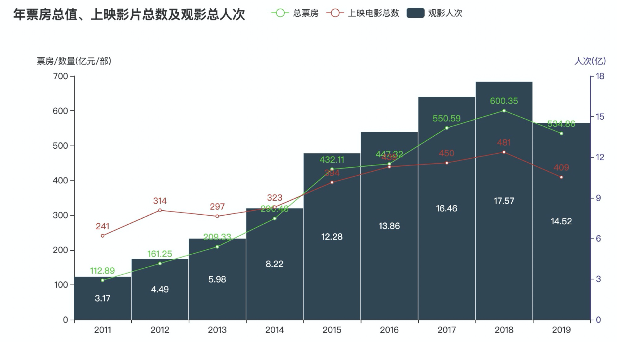
Figure 3 total box office and daily average box office
The release period of the film varies, which also affects the box office situation of the film, so we need to see the overall box office and daily box office situation of the single film in this picture.
config = {...} # db configuration omitted
conn = pymysql.connect(**config)
cursor = conn.cursor()
sql2 = '''select a.*,b.releasemonth from
(select movieid,
moviename,
round(sum(boxinfo)/10000,2) sumBox,
count(movieid) releasedays,
round(sum(boxinfo)/count(movieid)/10000,2) avgdaybox
from movies_data
where (substr(`releaseInfo`,1,2) = 'Release' or `releaseInfo`='Point projection' )
group by movieid,moviename) a ,
(select substr(date,5,2) releasemonth,movieId,movieName,releaseInfo from movies_data where releaseInfo='First day of release') b
where a.movieid = b.movieid order by sumBox desc'''
cursor.execute(sql2)
data3 = cursor.fetchall()
x_data3 = [i[1] for i in data3[:30]] # Name
y_data3_1 = [i[2] for i in data3[:30]] # Total box office
y_data3_2 = [i[4] for i in data3[:30]] # Average daily box office
y_data3_3 = [int(i[5]) for i in data3[:30]] # Show month
cursor.close()
conn.close()
def bar_base() -> Line:
c = (
Bar(init_opts=opts.InitOpts(height="600px", width="1500px"))
.add_xaxis(x_data3)
.add_yaxis("Total box office", y_data3_1, yaxis_index=0)
# . add yaxis ("daily box office of film", y data3 2, yaxis index = 1, gap = '- 40%')
.set_global_opts(title_opts=opts.TitleOpts(title="Total box office and daily average box office"),
xaxis_opts=opts.AxisOpts(axislabel_opts=opts.LabelOpts(rotate=-45)),
datazoom_opts=opts.DataZoomOpts(), )
.set_series_opts(label_opts=opts.LabelOpts(is_show=False), # Do not display dimensions on columns (numeric)
markpoint_opts=opts.MarkPointOpts(
data=[opts.MarkPointItem(type_="max", name="Maximum value"),
opts.MarkPointItem(type_="min", name="minimum value"), ]),)
.extend_axis(
yaxis=opts.AxisOpts(name="Billion yuan", position='left'))
.extend_axis(
yaxis=opts.AxisOpts(name="Billion yuan", type_="value", position="right", # Set the name, type and position of y-axis
axisline_opts=opts.AxisLineOpts(linestyle_opts=opts.LineStyleOpts(color="#483D8B")), ))
)
bar = (
Bar(init_opts=opts.InitOpts(height="600px", width="1500px"))
.add_xaxis(x_data3)
# . add yaxis ("total box office of films", y data3 1, yaxis index = 0)
.add_yaxis("Daily box office", y_data3_2, yaxis_index=2, gap='-40%')
.set_global_opts(title_opts=opts.TitleOpts(title="Total box office and daily average box office"),)
.set_series_opts(label_opts=opts.LabelOpts(is_show=False), # Do not display dimensions on columns (numeric)
markpoint_opts=opts.MarkPointOpts(
data=[opts.MarkPointItem(type_="max", name="Maximum value"),
opts.MarkPointItem(type_="min", name="minimum value"), ]),
markline_opts=opts.MarkLineOpts(
data=[opts.MarkLineItem(type_="average", name="average value"), ]
),)
)
c.overlap(bar)
return Grid().add(c, opts.GridOpts(pos_left="5%", pos_right="20%"), is_control_axis_index=True) # Adjusting position
bar_base().render("v3.html")
It can be seen that although the total box office of some films is average, the daily box office is very high, indicating that the release time is not long, but it is very popular.
However, for films with high total box office but average daily box office, it may be due to the longer release time and the lower attendance rate in the later stage that lower the average daily box office.
So to see the popularity of a movie, the total box office is only one aspect, and the trend of attendance change within the same release time is also very important.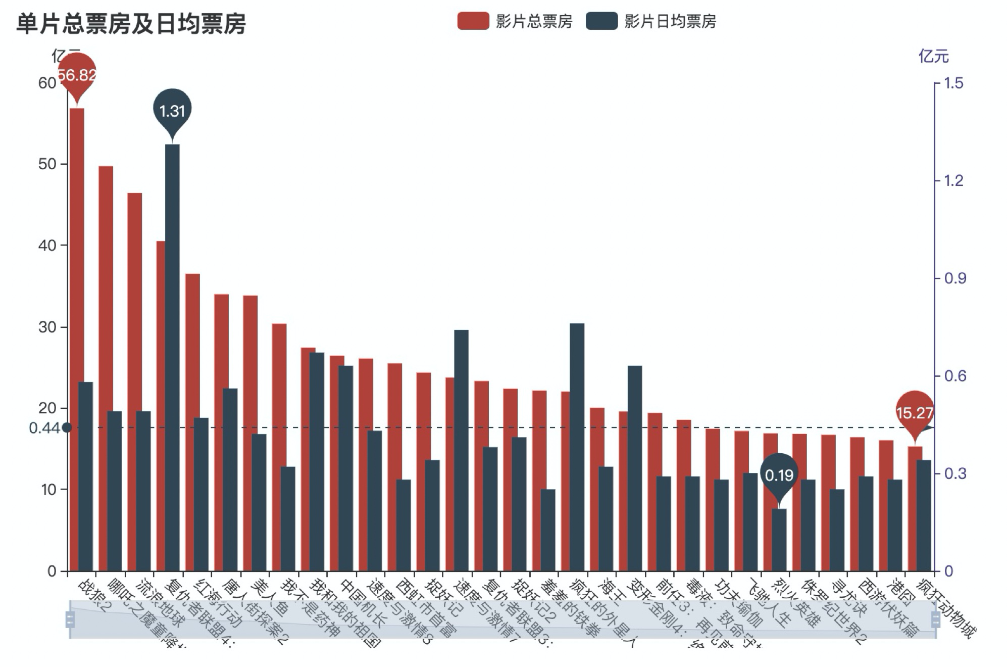
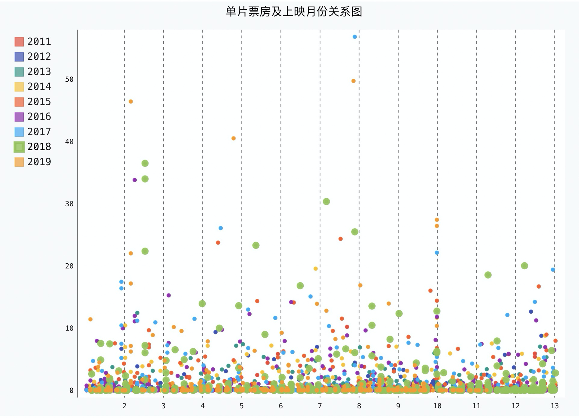
Figure 4 Relationship between single ticket office and release month
This picture is equivalent to the supplement of Figure 1, mainly to see the relationship between high box office movies and release time
def dayformat(i):
    mm = int(i[-2])
    dd = int(i[-1])
    mmdd = mm + dd/100*3.3
    return mmdd

config = {...}    # db configuration omitted
conn = pymysql.connect(**config)

cursor = conn.cursor()
sql2 = '''select a.*,b.releaseyear,b.releasemonth,b.releaseday from
            (select movieid,
                    moviename,
                    round(sum(boxinfo)/10000,2) sumBox,
                    count(movieid) releasedays,
                    round(sum(boxinfo)/count(movieid)/10000,2) avgdaybox
            from movies_data
            where (substr(`releaseInfo`,1,2) = 'Release' or `releaseInfo`='Point projection' )
            group by movieid,moviename) a ,
            (select substr(date,1,4) releaseyear,
                    substr(date,5,2) releasemonth,
                    substr(date,7,2) releaseday,
                    movieId,
                    movieName,
                    releaseInfo
                from movies_data where releaseInfo='First day of release') b
        where a.movieid = b.movieid  order by sumBox desc'''

cursor.execute(sql2)
data4 = cursor.fetchall()

x_data4 = [i for i in range(1, 13)]
y_data4_1 = [(dayformat(i), i[2]) for i in data4 if i[-3] == '2011']
y_data4_2 = [(dayformat(i), i[2]) for i in data4 if i[-3] == '2012']
y_data4_3 = [(dayformat(i), i[2]) for i in data4 if i[-3] == '2013']
y_data4_4 = [(dayformat(i), i[2]) for i in data4 if i[-3] == '2014']
y_data4_5 = [(dayformat(i), i[2]) for i in data4 if i[-3] == '2015']
y_data4_6 = [(dayformat(i), i[2]) for i in data4 if i[-3] == '2016']
y_data4_7 = [(dayformat(i), i[2]) for i in data4 if i[-3] == '2017']
y_data4_8 = [(dayformat(i), i[2]) for i in data4 if i[-3] == '2018']
y_data4_9 = [(dayformat(i), i[2]) for i in data4 if i[-3] == '2019']
cursor.close()
conn.close()

my_config = pygal.Config()  # Create Config instance
my_config.show_y_guides = False  # Hide horizontal dashes
my_config.show_x_guides = True
xy_chart = pygal.XY(stroke=False, config=my_config)
xy_chart.title = 'Relationship between single box office and release month'

xy_chart.add('2011', y_data4_1)
xy_chart.add('2012', y_data4_2)
xy_chart.add('2013', y_data4_3)
xy_chart.add('2014', y_data4_4)
xy_chart.add('2015', y_data4_5)
xy_chart.add('2016', y_data4_6)
xy_chart.add('2017', y_data4_7)
xy_chart.add('2018', y_data4_8)
xy_chart.add('2019', y_data4_9)


xy_chart.render_to_file("v4.svg")
The last part [python data analysis practice] box office data analysis (I) data collection