Python data analysis and presentation

Keywords: Python

Python data analysis and presentation

0.conda and IPython

anaconda=conda + Python of a certain version + third-party library

conda: package and environment management tools

IPython

？

Add a before or after the variable? Display general information

%Command

command	meaning
%run	Execute% (execute external code) in an empty namespace
%magic	Show all magic commands
%hist	IPython command input history
%pdb	Automatically enter the debugger after an exception occurs
%reset	Empty namespace
%who	Displays the variables defined in the namespace
%time statement	Give code execution time
%timeit statement	Execute the code multiple times and calculate the comprehensive average execution time
%paste/%cpaste	Don't mess the format when copying code
%timeit	Calculate code run time

1.Numpy Library

Difference between list and array

The list data types can be different, and the array data types are the same

N-dimensional array object: ndarray

The bottom layer of numpy is implemented by C
np.array() generates an array of ndarray s
axis: the dimension to save data
rank: number of dimensions (number of axes)

ndarray object properties

attribute	explain
.ndim	Number of dimensions (number of axes)
.shape	The scale of ndarray is n rows and m columns for a matrix
.size	Number of ndarray elements, equivalent to n*m in. shape
.dtype	ndarray element type
.itemsize	The size of the ndarray element in bytes

ndarray element type

data type	explain
bool	True or False
intc	Same as int (32 or 64) in C language
intp	Integer used for index, the same as ssize in C_ T (32 or 64)
int8	8-bit int
int16	16 bit int
int32	32-bit int
int64	64 bit int
uint8	8-bit unsigned
uint16	16 bit unsigned
uint32	32-bit unsigned
uint64	64 bit unsigned
float16	1+5+10
float32	1+8+23
float64	1+11+52
complex64	The complex number, real part and imaginary part are 32-bit floating-point numbers
complex128	The complex number, real part and imaginary part are 64 bit floating-point numbers

Create method

(1) Create ndarray from list, tuple

#list
>>> x=np.array([0,1,2,3])
>>> x
array([0, 1, 2, 3])
#tuple
>>> x=np.array((1,2,3))
>>> x
array([1, 2, 3])
#List tuple mixing
>>> x=np.array([[1,2],[9,8],(0.1,0.2)])
>>> x
array([[1. , 2. ],
       [9. , 8. ],
       [0.1, 0.2]])

(2) Functions provided by Numpy

function	explain
np.arange(n)	Returns ndarray, from 0 to n-1
np.ones(shape)	Generate a full 1 array, and shape is a tuple
np.zeros(shape)	Generate all 0 arrays, and shape is a tuple
np.full(shape,val)	Generate a full val array. shape is a tuple
np.eye(n)	Generate n*n diagonal matrix
np.ones_like(a)	Generate a full 1 array according to the shape of A
np.zeros_like(a)	Generate an array of all zeros according to the shape of a
np.full_like(a,val)	Generate a full val array according to the shape of A

(3) Other functions

function	explain
np.linspace()	Fill the data evenly according to the start and end data to form an array
np.concatenate()	Merge two or more arrays

example:

>>> a=np.linspace(1,10,4)
>>> a
array([ 1.,  4.,  7., 10.])
>>> b=np.linspace(1,10,4,endpoint=False)
>>> b
array([1.  , 3.25, 5.5 , 7.75])
>>> c=np.concatenate((a,b))
>>> c
array([ 1.  ,  4.  ,  7.  , 10.  ,  1.  ,  3.25,  5.5 ,  7.75])

Dimension transformation

method	explain
.reshape(shape)	Without changing the original array, an array of shape shapes is returned according to the original array
.resize(shape)	Transform the original array into shape
.swapaxes(ax1,ax2)	Swap two of the n dimensions in the array
.flatten()	Returns the folded one-dimensional array without changing the original array

Array type transformation

>>> a=np.ones((2,3,4))
>>> a
array([[[1., 1., 1., 1.],
        [1., 1., 1., 1.],
        [1., 1., 1., 1.]],

       [[1., 1., 1., 1.],
        [1., 1., 1., 1.],
        [1., 1., 1., 1.]]])

>>> a=np.ones((2,3,4),dtype=np.int64)
>>> a
array([[[1, 1, 1, 1],
        [1, 1, 1, 1],
        [1, 1, 1, 1]],

       [[1, 1, 1, 1],
        [1, 1, 1, 1],
        [1, 1, 1, 1]]], dtype=int64)

>>> b=a.astype(np.float64)
>>> b
array([[[1., 1., 1., 1.],
        [1., 1., 1., 1.],
        [1., 1., 1., 1.]],

       [[1., 1., 1., 1.],
        [1., 1., 1., 1.],
        [1., 1., 1., 1.]]])

Array - > List

>>> a=np.full((2,3,4),25,dtype=np.int32)
>>> a
array([[[25, 25, 25, 25],
        [25, 25, 25, 25],
        [25, 25, 25, 25]],

       [[25, 25, 25, 25],
        [25, 25, 25, 25],
        [25, 25, 25, 25]]])
>>> a.tolist()
[[[25, 25, 25, 25], [25, 25, 25, 25], [25, 25, 25, 25]], [[25, 25, 25, 25], [25, 25, 25, 25], [25, 25, 25, 25]]]

Array index and slice

One dimensional array

>>> a=np.array([9,8,7,6,5])
>>> a[2]
7
>>> a[1:4:2]
array([8, 6])

Multidimensional array

>>> a=np.array([9,8,7,6,5])
>>> a[2]
7

>>> a[1:4:2]
array([8, 6])

>>> a=np.arange(24).reshape((2,3,4))
>>> a[1,2,3]
23

>>> a[:,1,-3]#Do not care about the first dimension. The second dimension is required to be 1 and the third dimension is - 3
array([ 5, 17])

>>> a[:,:,::2]#Do not care about the first and second dimensions, and the step size of the third dimension is 2
array([[[ 0,  2],
        [ 4,  6],
        [ 8, 10]],

       [[12, 14],
        [16, 18],
        [20, 22]]])

Array operation

>>> a=np.arange(24).reshape((2,3,4))
>>> a
array([[[ 0,  1,  2,  3],
        [ 4,  5,  6,  7],
        [ 8,  9, 10, 11]],

       [[12, 13, 14, 15],
        [16, 17, 18, 19],
        [20, 21, 22, 23]]])

>>> a=a/a.mean()
>>> a
array([[[0.        , 0.08695652, 0.17391304, 0.26086957],
        [0.34782609, 0.43478261, 0.52173913, 0.60869565],
        [0.69565217, 0.7826087 , 0.86956522, 0.95652174]],

       [[1.04347826, 1.13043478, 1.2173913 , 1.30434783],
        [1.39130435, 1.47826087, 1.56521739, 1.65217391],
        [1.73913043, 1.82608696, 1.91304348, 2.        ]]])

function	explain
np.abs(x) np.fabs(x)	Calculate the absolute value of each element of the array
np.sqrt(x)	Calculate the square root of each element of the array
np.square(x)	Calculate the square of each element of the array
np.log(x) np.log10(x) np.log2(x)	Calculate the natural logarithm, base 10 logarithm and base 2 logarithm of each element of the array
np.ceil(x) np.floor(x)	Calculate the ceiling value and floor value of each element of the array
np.rint(x)	Calculates the rounded value of each element of the array
np.modf(x)	Returns the decimal and integer parts of each element of the array as two independent arrays
np.cos(x) np.cosh(x) and so on	Calculate the trigonometric function and hyperbolic function of each element
np.exp(x)	Calculate the index value of each element of the array
np.sign(x)	Calculate the symbolic value of each element of the array 10
+ - * / **	Each element of the two arrays performs corresponding operation
np.maximum(x,y) np.fmax()	Calculation of maximum and minimum values at element level
np.copysign(x,y)	Assign the sign of each element value in array y to the corresponding element of array x
np.mod(x,y)	Modular operation at element level
> < >= <= == !=	Arithmetic comparison to produce Boolean arrays

>>> import numpy as np
>>> a=np.arange(24).reshape((2,3,4))
>>> np.square(a)
array([[[  0,   1,   4,   9],
        [ 16,  25,  36,  49],
        [ 64,  81, 100, 121]],

       [[144, 169, 196, 225],
        [256, 289, 324, 361],
        [400, 441, 484, 529]]], dtype=int32)
>>> a=np.sqrt(a)
>>> a
array([[[0.        , 1.        , 1.41421356, 1.73205081],
        [2.        , 2.23606798, 2.44948974, 2.64575131],
        [2.82842712, 3.        , 3.16227766, 3.31662479]],

       [[3.464 one hundred and one 62, 3.60555128, 3.74165739, 3.87298335],
        [4.        , 4.12310563, 4.24264069, 4.35889894],
        [4.47213595, 4.58257569, 4.69041576, 4.79583152]]])
>>> np.modf(a)
(array([[[0.        , 0.        , 0.41421356, 0.73205081],
        [0.        , 0.23606798, 0.44948974, 0.64575131],
        [0.82842712, 0.        , 0.16227766, 0.31662479]],

       [[0.46410162, 0.60555128, 0.74165739, 0.87298335],
        [0.        , 0.12310563, 0.24264069, 0.35889894],
        [0.47213595, 0.58257569, 0.69041576, 0.79583152]]]), array([[[0., 1., 1., 1.],
        [2., 2., 2., 2.],
        [2., 3., 3., 3.]],

       [[3., 3., 3., 3.],
        [4., 4., 4., 4.],
        [4., 4., 4., 4.]]]))

>>> a=np.arange(24).reshape((2,3,4))
>>> b=np.sqrt(a)
>>> a
array([[[ 0,  1,  2,  3],
        [ 4,  5,  6,  7],
        [ 8,  9, 10, 11]],

       [[12, 13, 14, 15],
        [16, 17, 18, 19],
        [20, 21, 22, 23]]])
>>> b
array([[[0.        , 1.        , 1.41421356, 1.73205081],
        [2.        , 2.23606798, 2.44948974, 2.64575131],
        [2.82842712, 3.        , 3.16227766, 3.31662479]],

       [[3.46410162, 3.60555128, 3.74165739, 3.87298335],
        [4.        , 4.12310563, 4.24264069, 4.35889894],
        [4.47213595, 4.58257569, 4.69041576, 4.79583152]]])
>>> np.maximum(a,b)
array([[[ 0.,  1.,  2.,  3.],
        [ 4.,  5.,  6.,  7.],
        [ 8.,  9., 10., 11.]],

       [[12., 13., 14., 15.],
        [16., 17., 18., 19.],
        [20., 21., 22., 23.]]])
>>> a>b
array([[[False, False,  True,  True],
        [ True,  True,  True,  True],
        [ True,  True,  True,  True]],

       [[ True,  True,  True,  True],
        [ True,  True,  True,  True],
        [ True,  True,  True,  True]]])

Write csv

np.savetxt(fname,array,fmt='%.18e',delimiter=None)

frame: file, string or generator, which can be a compressed file of. gz or. bz2
Array: the array stored in the file
fmt: the format in which the file is written, e.g.% d,%.2f,%.18e
delimiter: splits a string. The default is a space

a=np.array(100).reshape(5,20)
np.savetxt('a.csv',a,fmt='%d',delimiter=',')
0,1,2,3...99

a=np.array(100).reshape(5,20)
np.savetxt('a.csv',a,fmt='%1f',delimiter=',')
0.0,1.0,2.0...99.0

Read csv

np.loadtxt(fname,dtype=np.float,delimiter=None,unpack=False)

frame: file, string or generator, which can be a compressed file of. gz or. bz2
dtype: data type; optional
delimiter: split string, default space
unpack: if True, the read in properties will be written to different variables respectively

b=np.loadtxt('a.csv',delimiter=',')
b=np.loadtxt('a.csv',dtype=int,delimiter=',')

Multidimensional data access

The above savetxt and loadtext can only handle one-dimensional and two-dimensional arrays

a.tofile(fname,sep='',format='%s')

frame: file, string
sep: data split string. If it is an empty string, the written file is binary
Format: the format of the written data

a=np.arange(100).reshape(5,10,2)
a.tofile('b.dat',sep=',',format='%d')
#Generating binaries without specifying sep

np.fromfile(fname,dtype=float,count=-1,sep='')

frame: file, string
dtype: read data type
count: the number of elements read in, - 1 means the whole file is read in
sep: data split string. If it is an empty string, the written file is binary

a=np.arange(100).reshape(5,10,2)
a.tofile('b.dat',sep=',',format='%d')
c=np.fromfile('b.dat',dtype=np.int,sep=",")
c=np.fromfile('b.dat',dtype=np.int,sep=",").reshape(5,10,2)

Convenient file access

np.save(fname,array)

np.savez(fname,array)

np.load(fname)

fname: file name, with. npy as the extension and npz as the compression extension
Array: array variable

a=np.arange(100).reshape(5,10,2)
np.save("a.npy",a)
b=np.load("a.npy")

Random number function

function	explain
rand(d0,d1...dn)	Create a random number array according to d0 DN, floating point number [0,1], evenly distributed
randn(d0,d1...dn)	Create a random number array according to d0 DN, with standard normal distribution
randint(low[,high,shape])	Create random integers or array of integers according to shape (the range is [low,high)
seed(s)	Random number seed, s is the given seed value

>>> a=np.random.rand(3,4,5)
>>> a
array([[[0.31789129, 0.04067915, 0.83303674, 0.68403089, 0.8170608 ],
        [0.48896229, 0.87662241, 0.80402316, 0.65002092, 0.60505475],
        [0.15862944, 0.86727453, 0.52962166, 0.60726439, 0.82176069],
        [0.12508611, 0.42132045, 0.31606682, 0.35658386, 0.19045285]],

       [[0.89511544, 0.26119674, 0.64866715, 0.23401689, 0.95676794],
        [0.43291969, 0.6155749 , 0.92665404, 0.05817955, 0.51062756],
        [0.10594579, 0.73809733, 0.47707574, 0.07499143, 0.11235247],
        [0.1250221 , 0.7002249 , 0.69170791, 0.74646681, 0.63357624]],

       [[0.50299485, 0.67903174, 0.73188944, 0.6296878 , 0.98629917],
        [0.8952625 , 0.76823821, 0.48124231, 0.02401954, 0.41473022],
        [0.72505748, 0.31233367, 0.81575195, 0.19943229, 0.60471366],
        [0.90742952, 0.89124879, 0.1213489 , 0.88284548, 0.67810859]]])

>>> sn=np.random.randn(3,4,5)
>>> sn
array([[[ 1.1832839 ,  0.25060466, -0.57017814,  0.47517595,
         -1.51740385],
        [ 0.35038796, -1.82168871,  0.16061641, -0.88696559,
          0.94106256],
        [ 0.77097301,  1.11086675,  0.32795292, -0.9581694 ,
         -1.75591931],
        [-0.14176509,  1.68687842,  1.30323321,  0.30734734,
         -0.42623733]],

       [[ 1.00836129, -1.4763877 , -0.10079373, -0.631505  ,
         -0.33870885],
        [-0.88316216, -1.5023321 , -0.51582272,  0.46557721,
          1.47694773],
        [-0.4808448 ,  0.88825249, -0.07169483, -0.03960847,
          2.03167751],
        [ 1.38474762,  0.86621196,  0.68230671, -0.75887396,
         -0.41100159]],

       [[-0.18006775,  0.50978947, -0.2241126 , -1.37232262,
          0.74588361],
        [-0.77222672,  0.06994181, -0.23934626,  0.43249514,
          0.40141005],
        [-1.35859946,  1.47103075,  0.59458256, -1.81122503,
          0.93659709],
        [-0.80001237, -0.46711391,  0.70415531,  0.2639113 ,
         -0.17576713]]])

>>> b=np.random.randint(100,200,(3,4))
>>> b
array([[164, 145, 135, 156],
       [161, 165, 199, 132],
       [182, 192, 155, 178]])

>>> import numpy as np
>>> np.random.seed(10)
>>> np.random.randint(100,200,(3,4))
array([[109, 115, 164, 128],
       [189, 193, 129, 108],
       [173, 100, 140, 136]])
>>> np.random.randint(100,200,(3,4))
array([[116, 111, 154, 188],
       [162, 133, 172, 178],
       [149, 151, 154, 177]])
>>> np.random.seed(10)
>>> np.random.randint(100,200,(3,4))
array([[109, 115, 164, 128],
       [189, 193, 129, 108],
       [173, 100, 140, 136]])

function	explain
shuffle(a)	Randomly arrange according to the first axis of array a and change array x
permutation(a)	Generate a new out of order array according to the first axis of array a without changing array x
choice(a[,size,replace,p])	Extract elements from one-dimensional array a with probability p to form a new array of size shape. replace indicates whether elements can be reused. The default is True

shuffle demo

>>> b=np.random.randint(100,200,(3,4))
>>> b
array([[164, 145, 135, 156],
       [161, 165, 199, 132],
       [182, 192, 155, 178]])
>>> a=np.random.randint(100,200,(3,4))
>>> a
array([[144, 104, 103, 126],
       [156, 145, 190, 195],
       [184, 186, 183, 160]])
>>> np.random.shuffle(a)
>>> a
array([[144, 104, 103, 126],
       [184, 186, 183, 160],
       [156, 145, 190, 195]])
>>> np.random.shuffle(a)
>>> a
array([[156, 145, 190, 195],
       [184, 186, 183, 160],
       [144, 104, 103, 126]])

permutation demo

>>> a=np.random.randint(100,200,(3,4))
>>> a
array([[138, 174, 192, 151],
       [171, 109, 107, one hundred and twenty-seven],
       [144, 174, 151, 138]])
>>> np.random.permutation(a)
array([[171, 109, 107, one hundred and twenty-seven],
       [144, 174, 151, 138],
       [138, 174, 192, 151]])
>>> a
array([[138, 174, 192, 151],
       [171, 109, 107, 127],
       [144, 174, 151, 138]])

choice demo

>>> b=np.random.randint(100,200,(8,))
>>> b
array([181, 106, 171, 103, 198, 168, 180, 192])
>>> np.random.choice(b,(3,2),replace=False)
array([[106, 168],
       [198, 180],
       [192, 103]])
>>> np.random.choice(b,(3,2),p=b/np.sum(b))
array([[168, 168],
       [192, 171],
       [192, 168]])

function	explain
uniform(low,high,size)	Generate a uniformly distributed array, with low as the starting value, high as the ending value and size as the shape
normal(loc,scale,size)	Generate a normal distribution array, loc is the mean, scale is the standard deviation, and size is the shape
poisson(lam,size)	Generate a Poisson distribution array, lam is the probability of random events, and size is the shape

>>> u=np.random.uniform(0,10,(3,4))
>>> u
array([[8.73861146, 0.46324114, 6.75838186, 0.71928162],
       [5.3382006 , 5.31719917, 9.72423284, 0.74520933],
       [2.51992423, 2.65729896, 1.41524432, 5.0901383 ]])
>>> n=np.random.normal(10,5,(3,4))
>>> n
array([[ 7.96208063, 20.35050238, 12.34165304,  6.72274216],
       [24.59582282,  9.98507963,  9.87675547,  6.42073446],
       [13.78549274,  7.68922186, 10.98222814,  5.73539134]])

Statistical function

function	explain
sum(a,axis=None)	Calculate the sum of the related elements of array a according to the given axis, axis integer or tuple
mean(a,axis=None)	Calculate the related elements of array a according to the given axis, and expect axis integer or tuple
average(a,axis=None,weights=None)	Calculate the weighted average of the relevant elements of array a according to the given axis
std(a,axis=None)	Calculate the standard deviation of relevant elements of array a according to the given axis
var(a,axis=None)	Calculate the variance of related elements of array a according to the given axis

>>> np.random.choice(b,(3,2),p=b/np.sum(b))
array([[168, 168],
       [192, 171],
       [192, 168]])
>>> u=np.random.uniform(0,10,(3,4))
>>> u
array([[8.73861146, 0.46324114, 6.75838186, 0.71928162],
       [5.3382006 , 5.31719917, 9.72423284, 0.74520933],
       [2.51992423, 2.65729896, 1.41524432, 5.0901383 ]])
>>> n=np.random.normal(10,5,(3,4))
>>> n
array([[ 7.96208063, 20.35050238, 12.34165304,  6.72274216],
       [24.59582282,  9.98507963,  9.87675547,  6.42073446],
       [13.78549274,  7.68922186, 10.98222814,  5.73539134]])
>>> a=np.arange(15).reshape(3,5)
>>> a
array([[ 0,  1,  2,  3,  4],
       [ 5,  6,  7,  8,  9],
       [10, 11, 12, 13, 14]])
>>> np.sum(a)
105
>>> np.mean(a,axis=1)
array([ 2.,  7., 12.])
>>> np.mean(a,axis=0)
array([5., 6., 7., 8., 9.])
>>> np.average(a,axis=0,weights=[10,5,1])
array([2.1875, 3.1875, 4.1875, 5.1875, 6.1875])
>>> np.std(a)
4.320493798938574
>>> np.var(a)
18.666666666666668

function	explain
min(a) max(a)	Calculates the minimum and maximum values of the elements in array a
argmin(a) argmax(a)	Calculate the subscript after one-dimensional reduction of the minimum and maximum values of elements in array a
unravel_index(index,shape)	Convert one-dimensional index into multi-dimensional index according to shape
ptp(a)	Calculates the difference between the maximum and minimum values of elements in array a
median(a)	Calculates the median of the elements in array a

>>> b=np.arange(15,0,-1).reshape(3,5)
>>> b
array([[15, 14, 13, 12, 11],
       [10,  9,  8,  7,  6],
       [ 5,  4,  3,  2,  1]])
>>> np.max(b)
15
>>> np.argmax(b)
0
>>> np.unravel_index(np.argmax(b),b.shape)
(0, 0)

Gradient function

np.gradient(f)

Calculate the gradient of elements in array F. when f is multidimensional, return the gradient of each dimension

>>> a=np.random.randint(0,20,(5))
>>> a
array([11,  3, 14, 18, 11])
>>> np.gradient(a)
array([-8. ,  1.5,  7.5, -1.5, -7. ])#1.5=(14-11)/2,-7=(11-18)/1
>>> b=np.random.randint(0,20,(5))
>>> b
array([15, 12, 19,  7, 15])
>>> np.gradient(b)
array([-3. ,  2. , -2.5, -2. ,  8. ])

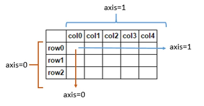
Understanding of axis

axis=0 removes the outermost parentheses and regards them as a whole. Operations are performed on this whole

axis=1 removes the second bracket and regards it as a whole. The operation is performed on this whole

... and so on

axis=0 means down, and axis=1 means across

A value of 0 means that the method is executed down the label \ index value of each column or row
A value of 1 indicates that the corresponding method is executed along the label direction of each row or column

Example: picture hand drawing effect

from PIL import Image
import numpy as np

a = np.asarray(Image.open('./beijing.jpg').convert('L')).astype('float')

depth = 10. 						# Preset depth value (0-100)
grad = np.gradient(a)				#Take the gradient value of image gray level
grad_x, grad_y = grad 				#Take the gradient values of horizontal and vertical images respectively
grad_x = grad_x*depth/100.
grad_y = grad_y*depth/100.          #Gradient normalization
A = np.sqrt(grad_x**2 + grad_y**2 + 1.)
uni_x = grad_x/A
uni_y = grad_y/A
uni_z = 1./A

vec_el = np.pi/2.2 					# Top view angle of light source, radian value
vec_az = np.pi/4. 					# Azimuth angle of light source, radian value
dx = np.cos(vec_el)*np.cos(vec_az) 	#Influence of light source on x-axis
dy = np.cos(vec_el)*np.sin(vec_az) 	#Influence of light source on y-axis
dz = np.sin(vec_el) 				#Influence of light source on z-axis

b = 255*(dx*uni_x + dy*uni_y + dz*uni_z) 	#Light source normalization
b = b.clip(0,255)

im = Image.fromarray(b.astype('uint8')) 	#Reconstructed image
im.save('./beijingHD.jpg')

2. Matlab Library

Basic operation

import matplotlib.pyplot as plt
plt.plot([0,2,4,6,8],[3,1,4,5,2])#If there is only one, it is regarded as the ordinate
plt.ylabel("grade")#Label
plt.savefig('test',dpi=600)#Store pictures
plt.axis([-1,10,0,6])#Horizontal axis range
plt.subplot(3,2,4)#It is divided into 3 * 2 sub drawing space and painted in the fourth space
plt.show()

plot() function

plt.plot(x,y,format_string,**kwargs)

x: X-axis data, list or array, can not be written
y: Y-axis data, list or array, must have
format_string: format string of control curve; optional
**kwargs: second group or more (x, y, format)_ string)
When drawing multiple curves, the x of each curve cannot be omitted

>>> import matplotlib.pyplot as plt
>>> import numpy as np
>>> a=np.arange(10)
>>> plt.plot(a,a*1.5,a,a*2.5,a,a*3.5,a,a*4.5)
[<matplotlib.lines.Line2D object at 0x000002BABE2752E0>, <matplotlib.lines.Line2D object at 0x000002BABE275160>, <matplotlib.lines.Line2D object at 0x000002BABE275460>, <matplotlib.lines.Line2D object at 0x000002BABE2754F0>]
>>> plt.show()

format_string value: color character + style character + mark character

Color character	explain	Color character	explain
'b'	blue	'm'	Magenta
'g'	green	'y'	yellow
'r'	gules	'k'	black
'c'	Turquoise	'w'	white
'#008000'	RGB a color	'0.8'	Grayscale value string

Style character	explain
'-'	Solid line
'–'	Broken broken line
'-.'	Dotted line
':'	Dotted line
''''	Wireless strip

Marker character	explain	Marker character	explain	Marker character	explain
'.'	Point marker	'1'	Lower flower triangle mark	'h'	Vertical hexagon mark
','	Pixel marker	'2'	Flower triangle mark	'H'	Horizontal hexagon mark
'o'	Solid circle mark	'3'	Left flower triangle mark	'+'	Cross mark
'v'	Inverted triangle mark	'4'	Right flower triangle mark	'x'	x mark
'^'	Upper triangle mark	's'	Filled square marker	'D'	Diamond mark
'>'	Right triangle mark	'p'	Black pentagonal marker	'd'	Thin diamond marker
'<'	Left triangle mark	'*'	Star Mark	'\|'	Vertical line marking

>>> import matplotlib.pyplot as plt
>>> import numpy as np
>>> a=np.arange(10)
>>> plt.plot(a,a*1.5,'go-',a,a*2.5,'rx',a,a*3.5,'*',a,a*4.5,'b-.')
[<matplotlib.lines.Line2D object at 0x000002BABAC37670>, <matplotlib.lines.Line2D object at 0x000002BABAC37730>, <matplotlib.lines.Line2D object at 0x000002BABAC37610>, <matplotlib.lines.Line2D object at 0x000002BABAC377C0>]
>>> plt.show()

**kwargs

Color: control color, color = "green"
linstyle: line style, linestyle = "dashed"
Marker: marker style, marker = 'o'
Markerfacecolor: marker color, markerfacecolor = 'blue'
Markersize: mark size, markersize=20

Chinese display (recommendation 2)

pylot does not support Chinese display by default

Rcparams (Global modification)

attribute	explain
'font.family'	The name used to display the font
'font.style'	The font style is normal, italic; italic
'font.size'	Font size, integer font size or 'large', 'x-small'

Chinese font	explain
'SimHei'	Chinese bold
'Kaiti'	Chinese regular script
'LiSu'	Chinese official script
'FangSong'	Chinese imitation Song Dynasty
'YouYuan'	Chinese immature circle
'STSong'	Chinese Song typeface

import matplotlib.pyplot as plt
import matplotlib
matplotlib.rcParams['font.family']='SimHei'
plt.plot([3,1,4,5,2])
plt.ylabel("Longitudinal axis (value)")
plt.savefig('test',dpi=600)
plt.show()

import matplotlib.pyplot as plt
import matplotlib
import numpy as np

matplotlib.rcParams['font.family']='Microsoft YaHei'
matplotlib.rcParams['font.size']=20
a=np.arange(0.0,5.0,0.02)
plt.xlabel('Horizontal axis: time')
plt.ylabel('Longitudinal axis: amplitude')
plt.plot(a,np.cos(2*np.pi*a),'r--')
plt.show()

Fontproperties (local modification)

import matplotlib.pyplot as plt
import numpy as np

a=np.arange(0.0,5.0,0.02)
plt.xlabel('Horizontal axis: time',fontproperties='SimHei',fontsize=20)
plt.ylabel('Longitudinal axis: amplitude',fontproperties='SimHei',fontsize=20)
plt.plot(a,np.cos(2*np.pi*a),'r--')
plt.show()

Text display

function	explain
plt.xlabel()	Add a text label to the x-axis
plt.ylabel()	Add a text label to the y-axis
plt.title()	Add text labels to the graphics as a whole
plt.text()	Add text anywhere
plt.annotate()	Add notes with arrows in the drawing

import matplotlib.pyplot as plt
import numpy as np

a=np.arange(0.0,5.0,0.02)
plt.plot(a,np.cos(2*np.pi*a),'r--')

plt.xlabel('Horizontal axis: time',fontproperties='SimHei',fontsize=20,color='green')
plt.ylabel('Longitudinal axis: amplitude',fontproperties='SimHei',fontsize=20)
plt.title(r'Sine wave example $y=cos(2\pi x)$',fontproperties='SimHei',fontsize=20)
plt.text(2,1,r'$\mu=100$',fontsize=15)

plt.axis([-1,6,-2,2])
plt.grid(True)
plt.show()

import matplotlib.pyplot as plt
import numpy as np

a=np.arange(0.0,5.0,0.02)
plt.plot(a,np.cos(2*np.pi*a),'r--')

plt.xlabel('Horizontal axis: time',fontproperties='SimHei',fontsize=25,color='green')
plt.ylabel('Longitudinal axis: amplitude',fontproperties='SimHei',fontsize=25)
plt.title(r'Sine wave example $y=cos(2\pi x)$',fontproperties='SimHei',fontsize=25)
plt.annotate(r'$\mu=100$',xy=(2,1),xytext=(3,1.5),arrowprops=dict(facecolor='black',shrink=0.1,width=2))

plt.axis([-1,6,-2,2])
plt.grid(True)
plt.show()

Sub drawing area

plt.subplot2grid(GridSpec,CurSpec,colspan=1,rowspan=1)

GridSpec is a tuple that describes the partition of the sketchpad
CurSpec is a tuple, making a grid
colspan represents the extension of the column
rowspan represents an extension of a row

plt.subplot2grid((3,3),(0,0),colspan=3)
plt.subplot2grid((3,3),(1,0),colspan=2)
plt.subplot2grid((3,3),(1,2),rowspan=2)
plt.subplot2grid((3,3),(2,0))
plt.subplot2grid((3,3),(2,1))

import matplotlib.gridspec as gridspec
import matplotlib.pyplot as plt

gs=gridspec.GridSpec(3,3)
ax1=plt.subplot(gs[0:,])
ax2=plt.subplot(gs[1:-1])
ax3=plt.subplot(gs[1:,-1])
ax4=plt.subplot(gs[2,0])
ax5=plt.subplot(gs[2,1])

Basic chart function

function	explain
plt.plot(x,y,fmt,...)	Coordinate diagram
plt.boxplot(data,notch,position)	Box diagram
plt.bar(left,height,width,bottom)	Bar chart
plt.barh(width,bottom,left,height)	Horizontal bar chart
plt.polar(theta,r)	Polar diagram
plt.pie(data,explode)	Pie chart
plt.psd(x,NFFT=256,pad_to,F)	Power spectral density diagram
plt.specgram(x,NFFT=256,pad_to.F)	Spectrogram
plt.cohere(x,y,NFFT=256,Fs)	x-y correlation function
plt.scatter(x,y)	Scatter plot where xy is the same length
plt.step(x,y,where)	Step diagram
plt.hist(x,bins,normed)	histogram

Pie chart

import matplotlib.pyplot as pltlabels='frogs','hogs','dogs','logs'size=[15,30,45,10]explode=(0,0.1,0,0)plt.pie(size,explode=explode,labels=labels,autopct='%1.1f%%',shadow=False,startangle=90)plt.axis('equal')plt.show()

histogram

import matplotlib.pyplot as pltimport numpy as npnp.random.seed(0)mu,sigma=100,20a=np.random.normal(mu,sigma,size=100)plt.hist(a,20,density=True,histtype='stepfilled',facecolor='b',alpha=0.75)#density normalization plt.title('Histogram')plt.show()

Polar diagram

import matplotlib.pyplot as pltimport numpy as npN=20theta=np.linspace(0.0,2*np.pi,N,endpoint=False)radii=10*np.random.rand(N)width=np.pi/4*np.random.rand(N)ax=plt.subplot(111,projection='polar')#Create polar subgraph bars=ax.bar(theta,radii,width=width,bottom=0.0)#theta, radio, width corresponds to left, height, width for R, bar in zip (radio, bars): bar.set_ facecolor(plt.cm.viridis(r/10.))    bar.set_ alpha(0.5)plt.show()

Scatter diagram

import matplotlib.pyplot as pltimport numpy as npfig,ax=plt.subplots()ax.plot(10*np.random.randn(100),10*np.random.randn(100),'o')ax.set_title('Simple Scatter')plt.show()

3.Pandas Library

Two data types: series and dataframe

Series type

Custom index

It is composed of a set of data and its related indexes. It allows user-defined indexes

>>> import pandas as pd
>>> a=pd.Series([9,8,7,6])
>>> a
0    9
1    8
2    7
3    6
dtype: int64
>>> b=pd.Series([9,8,7,6],index=['a','b','c','d'])
>>> b
a    9
b    8
c    7
d    6
dtype: int64

establish

Python list

Scalar value

>>> s=pd.Series(25,index=['a','b','c'])#The index here cannot be omitted
>>> s
a    25
b    25
c    25
dtype: int64

Python dictionary

>>> d=pd.Series({'a':9,'b':8,'c':7})
>>> d
a    9
b    8
c    7
dtype: int64
    
>>> e=pd.Series({'a':9,'b':8,'c':7},index=['c','a','b','d'])#Select from the dictionary
>>> e
c    7.0
a    9.0
b    8.0
d    NaN
dtype: float64

ndarray

>>> import pandas as pd
>>> import numpy as np
>>> n=pd.Series(np.arange(5))
>>> n
0    0
1    1
2    2
3    3
4    4
dtype: int32

>>> m=pd.Series(np.arange(5),index=np.arange(9,4,-1))
>>> m
9    0
8    1
7    2
6    3
5    4
dtype: int32

Other functions

basic operation

Similar to ndarray, dictionary

>>> import pandas as pd
>>> b=pd.Series([9,8,7,6],['a','b','c','d'])
>>> b
a    9
b    8
c    7
d    6
dtype: int64
>>> b.index
Index(['a', 'b', 'c', 'd'], dtype='object')
>>> b.values
array([9, 8, 7, 6], dtype=int64)

>>> b['b']8>>> b[1]8>>> b[['c','d',0]]#Either of the two lassos can be referenced, but cannot be mixed > > > b [['C','d ',' a ']]c 7d 6a 9dtype: Int64

The Series operation is similar to the ndarray type

The index method is the same, []
Operations and operations in Numpy are available for Series types
You can slice through a list of custom indexes
It can be sliced through automatic index. If there is a custom index, it will be sliced together

>>> import pandas as pd>>> b=pd.Series([9,8,7,6],['a','b','c','d'])>>> ba    9b    8c    7d    6dtype: int64>>> b[3]6>>> b[:3]a    9b    8c    7dtype: int64>>> b[b>b.median()]a    9b    8dtype: int64>>> np.exp(b)a    8103.083928b    2980.957987c    1096.633158d     403.428793dtype: float64

The Series type operation is similar to the Python dictionary type

Access through custom index
Reserved word in operation
Use the. get() method

>>> import pandas as pd>>> b=pd.Series([9,8,7,6],['a','b','c','d'])>>> b['b']8>>> 'c' in bTrue>>> 0 in bFalse>>> b.get('f',100)100

Series type alignment operation

>>> import pandas as pd>>> a=pd.Series([1,2,3],['c','d','e'])>>> b=pd.Series([9,8,7,6],['a','b','c','d'])>>> a+ba    NaNb    NaNc    8.0d    8.0e    NaNdtype: float64#The Series type automatically aligns the data of different indexes during operation

name attribute of Series type

>>> import pandas as pd>>> b=pd.Series([9,8,7,6],['a','b','c','d'])>>> b.name>>> b.name='Series object'>>> b.index.name='Index column'>>> b Index column a    9b    8c    7d    6Name: Series object, dtype: int64

Series objects can be modified at any time and take effect immediately

>>> import pandas as pd>>> b=pd.Series([9,8,7,6],['a','b','c','d'])>>> b['a']=15>>> b.name="series">>> ba    15b     8c     7d     6Name: series, dtype: int64>>> b.name="New Series">>> b['b','c']=20>>> ba    15b    20c    20d     6Name: New Series, dtype: int64

DataFrame type

Consists of a set of columns that share an index

Row index, column index, column index

Cross column operation axis=1

Cross row operation axis=0

establish

2D ndarray object

>>> import pandas as pd>>> import numpy as np>>> d=pd.DataFrame(np.arange(10).reshape(2,5))>>> d   0  1  2  3  4#Automatic column index, 01 on the left is automatic row index 0 0 0 1 2 3 41 5 6 7 8 9

A dictionary consisting of one-dimensional ndarray, list, dictionary, tuple, or Series

>>> import pandas as pd>>> dt={'one':pd.Series([1,2,3],index=['a','b','c']),'two':pd.Series([9,8,7,6],index=['a','b','c','d'])}>>> d=pd.DataFrame(dt)>>> d   one  two#Custom column index and custom row index a  1.0    9b  2.0    8c  3.0    7d  NaN    6>>> pd.DataFrame(dt,index=['b','c','d'],columns=['two','three'])   two three#The data is automatically supplemented according to the row index b 8 NANC 7 NAND 6 Nan

Create from a list type dictionary

>>> import pandas as pd>>> dl={'one':[1,2,3,4],'two':[9,8,7,6]}>>> d=pd.DataFrame(dl,index=['a','b','c','d'])>>> d   one  twoa    1    9b    2    8c    3    7d    4    6

example

>>> import pandas as pd>>> dl={'city':['Beijing','Shanghai','Guangzhou','Shenzhen','Shenyang'],        'Ring ratio':[101.5,101.2,101.3,102.0,100.1],        'Year on year':[120.7,127.3,119.4,140.9,101.4],        'Fixed base':[121.4,127.8,120.0,145.5,101.6]}>>> d=pd.DataFrame(dl,index=['c1','c2','c3','c4','c5'])>>> d    city     Ring ratio     Year on year     Fixed base c1  Beijing 101.5  120.7  121.4c2  Shanghai 101.2  127.3  127.8c3  Guangzhou 101.3  119.4  120.0c4  Shenzhen 102.0  140.9  145.5c5  Shenyang 100.1  101.4  101.6>>> d.indexIndex(['c1', 'c2', 'c3', 'c4', 'c5'], dtype='object')>>> d.columnsIndex(['city', 'Ring ratio', 'Year on year', 'Fixed base'], dtype='object')>>> d.valuesarray([['Beijing', 101.5, 120.7, 121.4],       ['Shanghai', 101.2, 127.3, 127.8],       ['Guangzhou', 101.3, 119.4, 120.0],       ['Shenzhen', 102.0, 140.9, 145.5],       ['Shenyang', 100.1, 101.4, 101.6]], dtype=object)>>> d['Year on year']c1    120.7c2    127.3c3    119.4c4    140.9c5    101.4Name: Year on year, dtype: float64>>> d.loc['c2']city       Shanghai Chain comparison    101.2 Year on year    127.3 Fixed base    127.8Name: c2, dtype: object>>> d['Year on year']['c2']127.3

Series
Other dataframes

operation

reindex

.reindex()Capable of changing or remaking Series and DataFrame Index of

>>> import pandas as pd>>> dl={'city':['Beijing','Shanghai','Guangzhou','Shenzhen','Shenyang'],'Ring ratio':[101.5,101.2,101.3,102.0,100.1],'Year on year':[120.7,127.3,119.4,140.9,101.4],'Fixed base':[121.4,127.8,120.0,145.5,101.6]}>>> d=pd.DataFrame(dl,index=['c1','c2','c3','c4','c5'])>>> d    city     Ring ratio     Year on year     Fixed base c1  Beijing 101.5  120.7  121.4c2  Shanghai 101.2  127.3  127.8c3  Guangzhou 101.3  119.4  120.0c4  Shenzhen 102.0  140.9  145.5c5  Shenyang 100.1  101.4  101.6>>> d=d.reindex(index=['c5','c4','c3','c2','c1'])>>> d    city     Ring ratio     Year on year     Fixed base c5  Shenyang 100.1  101.4  101.6c4  Shenzhen 102.0  140.9  145.5c3  Guangzhou 101.3  119.4  120.0c2  Shanghai 101.2  127.3  127.8c1  Beijing 101.5  120.7  121.4>>> d=d.reindex(columns=['city','Year on year','Ring ratio','Fixed base'])>>> d    city     Year on year     Ring ratio     Fixed base c5  Shenyang 101.4  100.1  101.6c4  Shenzhen 140.9  102.0  145.5c3  Guangzhou 119.4  101.3  120.0c2  Shanghai 127.3  101.2  127.8c1  Beijing 120.7  101.5  121.4

.reindex(index=None,columns=None,...)

parameter	explain
index,columns	New row column custom index
fill_value	In the re index, the value used to populate the missing location
method	Filling method, fill forward with fill and fill backward with bfill
limit	Maximum fill
copy	The default is True to generate a new object; When False, the old and new equality is not copied

>>> newc=d.columns.insert(4,'newly added')>>> newd=d.reindex(columns=newc,fill_value=200)>>> newd    city     Year on year     Ring ratio     Fixed base addition c5  Shenyang 101.4  100.1  101.6  200c4  Shenzhen 140.9  102.0  145.5  200c3  Guangzhou 119.4  101.3  120.0  200c2  Shanghai 127.3  101.2  127.8  200c1  Beijing 120.7  101.5  121.4  200

Index type operation

Index type: the indexes of Series and DataFrame are of index type, and the index object is of non modifiable type

Common methods of index type

method	explain
.append(idx)	Connect another Index object to generate a new Index object
.diff(idx)	Calculate the difference set to generate a new Index object
.intersection(idx)	Calculate intersection
union(idx)	Computational Union
.delete(loc)	Delete the element at loc location
.insert(loc,e)	Add an element e at loc

>>> d
    city     Year on year     Ring ratio     Fixed base
c5  Shenyang 101.4  100.1  101.6
c4  Shenzhen 140.9  102.0  145.5
c3  Guangzhou 119.4  101.3  120.0
c2  Shanghai 127.3  101.2  127.8
c1  Beijing 120.7  101.5  121.4
>>> nc=d.columns.delete(2)
>>> ni=d.index.insert(5,'c0')
>>> nd=d.reindex(index=ni,columns=nc,method='ffill')#Will report an error
>>> nd=d.reindex(index=ni,columns=nc).ffill()
>>> nd
    city     Year on year     Fixed base
c5  Shenyang 101.4  101.6
c4  Shenzhen 140.9  145.5
c3  Guangzhou 119.4  120.0
c2  Shanghai 127.3  127.8
c1  Beijing 120.7  121.4
c0  Beijing 120.7  121.4

Deletes the specified index object

. drop() can delete the row or column indexes specified by Series and DataFrame

>>> a=pd.Series([9,8,7,6],index=['a','b','c','d'])
>>> a
a    9
b    8
c    7
d    6
dtype: int64
>>> a.drop(['b','c'])
a    9
d    6
dtype: int64
>>> d
    city     Year on year     Ring ratio     Fixed base
c5  Shenyang 101.4  100.1  101.6
c4  Shenzhen 140.9  102.0  145.5
c3  Guangzhou 119.4  101.3  120.0
c2  Shanghai 127.3  101.2  127.8
c1  Beijing 120.7  101.5  121.4
>>> d.drop('c5')
    city     Year on year     Ring ratio     Fixed base
c4  Shenzhen 140.9  102.0  145.5
c3  Guangzhou 119.4  101.3  120.0
c2  Shanghai 127.3  101.2  127.8
c1  Beijing 120.7  101.5  121.4
>>> d.drop('Year on year',axis=1)
    city     Ring ratio     Fixed base
c5  Shenyang 100.1  101.6
c4  Shenzhen 102.0  145.5
c3  Guangzhou 101.3  120.0
c2  Shanghai 101.2  127.8
c1  Beijing 101.5  121.4

Data type operation

add , subtract , multiply and divide

>>> a=pd.DataFrame(np.arange(12).reshape(3,4))
>>> a
   0  1   2   3
0  0  1   2   3
1  4  5   6   7
2  8  9  10  11
>>> b=pd.DataFrame(np.arange(20).reshape(4,5))
>>> b
    0   1   2   3   4
0   0   1   2   3   4
1   5   6   7   8   9
2  10  11  12  13  14
3  15  16  17  18  19
>>> a+b
      0     1     2     3   4
0   0.0   2.0   4.0   6.0 NaN
1   9.0  11.0  13.0  15.0 NaN
2  18.0  20.0  22.0  24.0 NaN
3   NaN   NaN   NaN   NaN NaN
>>> a*b
      0     1      2      3   4
0   0.0   1.0    4.0    9.0 NaN
1  20.0  30.0   42.0   56.0 NaN
2  80.0  99.0  120.0  143.0 NaN
3   NaN   NaN    NaN    NaN NaN

Operation in method form

method	explain
.add(d,**argws)	Addition between types, optional parameters
.sub(d,**argws)	Inter type subtraction, optional parameters
.mul(d,**argws)	Inter type multiplication, optional parameters
.div(d,**argws)	Division between types, optional parameters

>>> a
   0  1   2   3
0  0  1   2   3
1  4  5   6   7
2  8  9  10  11
>>> b
    0   1   2   3   4
0   0   1   2   3   4
1   5   6   7   8   9
2  10  11  12  13  14
3  15  16  17  18  19
>>> b.add(a,fill_value=100)#Replace NAN first and then participate in the operation
       0      1      2      3      4
0    0.0    2.0    4.0    6.0  104.0
1    9.0   11.0   13.0   15.0  109.0
2   18.0   20.0   22.0   24.0  114.0
3  115.0  116.0  117.0  118.0  119.0
>>> a.mul(b,fill_value=0)
      0     1      2      3    4
0   0.0   1.0    4.0    9.0  0.0
1  20.0  30.0   42.0   56.0  0.0
2  80.0  99.0  120.0  143.0  0.0
3   0.0   0.0    0.0    0.0  0.0

Broadcast operation is performed between different dimensions, and one-dimensional Series participates in the operation on axis 1 by default

>>> b
    0   1   2   3   4
0   0   1   2   3   4
1   5   6   7   8   9
2  10  11  12  13  14
3  15  16  17  18  19
>>> c=pd.Series(np.arange(4))
>>> c
0    0
1    1
2    2
3    3
dtype: int32
>>> c-10
0   -10
1    -9
2    -8
3    -7
dtype: int32
>>> b-c#axis=1, cross column
      0     1     2     3   4
0   0.0   0.0   0.0   0.0 NaN
1   5.0   5.0   5.0   5.0 NaN
2  10.0  10.0  10.0  10.0 NaN
3  15.0  15.0  15.0  15.0 NaN

Make one-dimensional Series participate in axis 0 operation

>>> b
    0   1   2   3   4
0   0   1   2   3   4
1   5   6   7   8   9
2  10  11  12  13  14
3  15  16  17  18  19
>>> c
0    0
1    1
2    2
3    3
dtype: int32
>>> b.sub(c,axis=0)
    0   1   2   3   4
0   0   1   2   3   4
1   4   5   6   7   8
2   8   9  10  11  12
3  12  13  14  15  16

Comparison operation

>>> a=pd.DataFrame(np.arange(12).reshape(3,4))
>>> d=pd.DataFrame(np.arange(12,0,-1).reshape(3,4))
>>> a
   0  1   2   3
0  0  1   2   3
1  4  5   6   7
2  8  9  10  11
>>> d
    0   1   2  3
0  12  11  10  9
1   8   7   6  5
2   4   3   2  1
>>> a>d
       0      1      2      3
0  False  False  False  False
1  False  False  False   True
2   True   True   True   True
>>> a==d
       0      1      2      3
0  False  False  False  False
1  False  False   True  False
2  False  False  False  False

>>> a
   0  1   2   3
0  0  1   2   3
1  4  5   6   7
2  8  9  10  11
>>> c
0    0
1    1
2    2
3    3
dtype: int32
>>> a>c
       0      1      2      3
0  False  False  False  False
1   True   True   True   True
2   True   True   True   True
>>> c>0
0    False
1     True
2     True
3     True
dtype: bool

Characteristic analysis of pandas data

.sort_ The index () method sorts by index on the specified axis. The default is ascending

.sort_index(axis=0,ascending=True)

>>> b=pd.DataFrame(np.arange(20).reshape(4,5),index=['c','a','d','b'])
>>> b
    0   1   2   3   4
c   0   1   2   3   4
a   5   6   7   8   9
d  10  11  12  13  14
b  15  16  17  18  19
>>> b.sort_index()
    0   1   2   3   4
a   5   6   7   8   9
b  15  16  17  18  19
c   0   1   2   3   4
d  10  11  12  13  14
>>> b.sort_index(ascending=False)
    0   1   2   3   4
d  10  11  12  13  14
c   0   1   2   3   4
b  15  16  17  18  19
a   5   6   7   8   9

>>> b
    0   1   2   3   4
c   0   1   2   3   4
a   5   6   7   8   9
d  10  11  12  13  14
b  15  16  17  18  19
>>> c=b.sort_index(axis=1,ascending=False)
>>> c
    4   3   2   1   0
c   4   3   2   1   0
a   9   8   7   6   5
d  14  13  12  11  10
b  19  18  17  16  15
>>> c=c.sort_index()
>>> c
    4   3   2   1   0
a   9   8   7   6   5
b  19  18  17  16  15
c   4   3   2   1   0
d  14  13  12  11  10

.sort_ The values () method sorts values on the specified axis. The default is ascending

Series.sort_values(axis=0,ascending=True)DataFrame.sort_values(by,axis=0,ascending=True)

by: an index or index list on the axis

>>> b    0   1   2   3   4c   0   1   2   3   4a   5   6   7   8   9d  10  11  12  13  14b  15  16  17  18  19>>> c=b.sort_values(2,ascending=False)>>> c    0   1   2   3   4b  15  16  17  18  19d  10  11  12  13  14a   5   6   7   8   9c   0   1   2   3   4>>> c=c.sort_values('a',axis=1,ascending=False)>>> c    4   3   2   1   0b  19  18  17  16  15d  14  13  12  11  10a   9   8   7   6   5c   4   3   2   1   0

NaN put it last

Basic statistical analysis

For Series and DataFrame

method	explain
.sum()	Calculate the sum of data according to the 0 axis
.count()	Number of non NaN values
.mean() .median()	Calculate the arithmetic mean and arithmetic median of the data
.var() .std()	Calculate the variance and standard deviation of the data
.min() .max()	Calculate the minimum and maximum values of the data

Series only

method	explain
.argmin() .argmax()	Calculate the automatic index of the location where the maximum and minimum values of data are located
.idxmin() .idxmax()	Calculate the user-defined index where the maximum and minimum values of data are located

For Series and DataFrame types

method	explain
.describe()	Statistical summary for axis 0 (columns)

>>> a=pd.Series([9,8,7,6],index=['a','b','c','d'])
>>> a
a    9
b    8
c    7
d    6
dtype: int64
>>> a.describe()
count    4.000000
mean     7.500000
std      1.290994
min      6.000000
25%      6.750000
50%      7.500000
75%      8.250000
max      9.000000
dtype: float64
>>> type(a.describe())
<class 'pandas.core.series.Series'>
>>> a.describe()['count']
4.0
>>> a.describe()['max']
9.0

>>> b
    0   1   2   3   4
c   0   1   2   3   4
a   5   6   7   8   9
d  10  11  12  13  14
b  15  16  17  18  19
>>> b.describe()
               0          1          2          3          4
count   4.000000   4.000000   4.000000   4.000000   4.000000
mean    7.500000   8.500000   9.500000  10.500000  11.500000
std     6.454972   6.454972   6.454972   6.454972   6.454972
min     0.000000   1.000000   2.000000   3.000000   4.000000
25%     3.750000   4.750000   5.750000   6.750000   7.750000
50%     7.500000   8.500000   9.500000  10.500000  11.500000
75%    11.250000  12.250000  13.250000  14.250000  15.250000
max    15.000000  16.000000  17.000000  18.000000  19.000000
>>> type(b.describe())
<class 'pandas.core.frame.DataFrame'>
>>> b.describe().loc['max']
0    15.0
1    16.0
2    17.0
3    18.0
4    19.0
Name: max, dtype: float64
>>> b.describe()[2]
count     4.000000
mean      9.500000
std       6.454972
min       2.000000
25%       5.750000
50%       9.500000
75%      13.250000
max      17.000000
Name: 2, dtype: float64

Cumulative statistical analysis

method	explain
.cumsum()	The sum of the first 1, 2... n numbers is given in turn
.cumprod()	The product of the first 1, 2... n numbers is given in turn
.cummax()	The maximum values of the first 1, 2... n numbers are given in turn
.cummin()	The minimum values of the first 1, 2... n numbers are given in turn

>>> b
    0   1   2   3   4
c   0   1   2   3   4
a   5   6   7   8   9
d  10  11  12  13  14
b  15  16  17  18  19
>>> b.cumsum()
    0   1   2   3   4
c   0   1   2   3   4
a   5   7   9  11  13
d  15  18  21  24  27
b  30  34  38  42  46
>>> b.cumprod()
   0     1     2     3     4
c  0     1     2     3     4
a  0     6    14    24    36
d  0    66   168   312   504
b  0  1056  2856  5616  9576
>>> b.cummin()
   0  1  2  3  4
c  0  1  2  3  4
a  0  1  2  3  4
d  0  1  2  3  4
b  0  1  2  3  4
>>> b.cummax()
    0   1   2   3   4
c   0   1   2   3   4
a   5   6   7   8   9
d  10  11  12  13  14
b  15  16  17  18  19

Applicable to Series and DataFrame types, rolling calculation (window calculation)

method	explain
.rolling(w).sum()	Calculate the sum of adjacent w elements in turn
.rolling(w).mean()	Calculate the arithmetic mean of adjacent w elements in turn
.rolling(w).var()	Calculate the variance of adjacent w elements in turn
.rolling(w).std()	Calculate the standard deviation of adjacent w elements in turn
.rolling(w).min() .max()	Calculate the minimum and maximum values of adjacent w elements in turn

>>> b
    0   1   2   3   4
c   0   1   2   3   4
a   5   6   7   8   9
d  10  11  12  13  14
b  15  16  17  18  19
>>> b.rolling(2).sum()
      0     1     2     3     4
c   NaN   NaN   NaN   NaN   NaN
a   5.0   7.0   9.0  11.0  13.0
d  15.0  17.0  19.0  21.0  23.0#21=8+13
b  25.0  27.0  29.0  31.0  33.0
>>> b.rolling(3).sum()
      0     1     2     3     4
c   NaN   NaN   NaN   NaN   NaN
a   NaN   NaN   NaN   NaN   NaN
d  15.0  18.0  21.0  24.0  27.0
b  30.0  33.0  36.0  39.0  42.0#42=9+14+19

correlation analysis

Pearson correlation coefficient
r = ∑ i = 1 n ( x i − x ‾ ) ( y i − y ‾ ) ∑ i = 1 n ( x i − x ‾ ) 2 ∑ i = 1 n ( y i − y ‾ ) 2 r=\frac{\sum_{i=1}^n(x_i-\overline x)(y_i-\overline y)}{\sqrt{\sum _{i=1}^n(x_i-\overline x)^2}\sqrt{\sum _{i=1}^n(y_i-\overline y)^2}} r=∑i=1n(xi−x)2 ∑i=1n(yi−y)2 ∑i=1n(xi−x)(yi−y)

correlation coefficient	Degree of correlation
0.8-1.0	Extremely strong correlation
0.6-0.8	Strong correlation
0.4-0.6	Moderate correlation
0.2-0.4	Weak correlation
0.0-0.2	Very weak correlation or no correlation

For Series and DataFrame types

method	explain
.cov()	Calculate covariance matrix
.corr()	Calculate correlation coefficient matrix

>>> import pandas as pd
>>> hprice=pd.Series([3.04,22.93,12.75,22.6,12.33],index=['2008','2009','2010','2011','2012'])
>>> m2=pd.Series([8.18,18.38,9.13,7.82,6.69],index=['2008','2009','2010','2011','2012'])
>>> hprice.corr(m2)
0.5239439145220387

Posted by nloding on Mon, 06 Sep 2021 17:31:28 -0700

Programmer Group

Python data analysis and presentation

Python data analysis and presentation

0.conda and IPython

IPython

？

%Command

1.Numpy Library

Difference between list and array

N-dimensional array object: ndarray

ndarray object properties

ndarray element type

Create method

Dimension transformation

Array type transformation

Array - > List

Array index and slice

Array operation

Write csv

Read csv

Multidimensional data access

Convenient file access

Random number function

Statistical function

Gradient function

Understanding of axis

Example: picture hand drawing effect

2. Matlab Library

Basic operation

plot() function

Chinese display (recommendation 2)

Text display

Sub drawing area

Basic chart function

3.Pandas Library

Series type

Custom index

establish

basic operation

DataFrame type

establish

operation

Index type operation

Data type operation

Characteristic analysis of pandas data

Basic statistical analysis

Cumulative statistical analysis

correlation analysis

Hot Keywords