The credit risk measurement model can include personal credit rating, enterprise credit rating and national credit rating. Human credit rating consists of A series of rating models, including A card (application scoring card), B card (behavior model), C card (collection model) and F card (anti fraud model). Today, we show the development process of personal credit rating model. The data adopts the well-known give me some credit data set on kaggle.
1, Project process
A typical credit scoring card model is shown in Figure 1-1. The main development process of credit risk rating model is as follows:
(1) Obtain data, including data of customers applying for loans. The data includes all dimensions of customers, including age, gender, income, occupation, number of families, housing, consumption, debt, etc.
(2) Data preprocessing mainly includes data cleaning, missing value processing, abnormal value processing, data type conversion and so on. We need to convert the original data layer by layer into modelable data.
(3) EDA exploratory data analysis and descriptive statistics, including the overall data volume, the proportion of good and bad customers, the types of data, the missing rate of variables, variable frequency analysis, histogram visualization, box chart visualization, variable correlation visualization, etc.
(4) Variable selection, through the methods of statistics and machine learning, select the variables that have the most significant impact on the default state. There are many common variable selection methods, including iv, feature importance, variance and so on. In addition, variables with high deletion rate are also recommended to be deleted. It is also recommended to delete if there are no business explanatory variables and no value variables.
(5) The main difficulties in model development and scorecard modeling are woe box division, score stretching and variable coefficient calculation. Among them, woe box division is the difficulty in the score card, which requires rich statistical knowledge and business experience. At present, there are more than 50 kinds of box splitting algorithms, and there is no unified gold standard. Generally, the machine automatically divides the box first, then manually adjusts the box splitting, and finally repeatedly tests the performance of the model and selects the best box splitting algorithm.
(6) Model verification: verify the discrimination ability, prediction ability, stability, sorting ability, etc. of the model, form a model evaluation report, and draw a conclusion whether the model can be used. Model validation is not completed at one time, but after modeling, before and after the model goes online. Model development and maintenance is a cycle, not completed at one time.
(7) The credit score card is generated according to the variable coefficient and WOE value of Logistic regression. The score card is convenient for business explanation. It has been used for decades and is very stable. It is deeply loved by the financial industry. The method is to convert the probability score of Logistic model into a standard score of 300-900.
(8) Scoring card automatic scoring system, according to the credit scoring card method, establish a computer automatic credit scoring system. FICO, a traditional American product, has similar functions. The underlying language of FICO is Java. At present, Java, python or R are popular to build scoring card automatic model system.
(9) Model monitoring, as time goes by, the model discrimination ability, such as KS and AUC, will gradually decline, and the model stability will shift. We need a professional model monitoring team. When it is monitored that the model differentiation ability decreases significantly or the model stability deviates greatly, we need to redevelop the model and iterate the model. The model monitoring team should send model monitoring reports to relevant teams on time every day, especially the development team and business team.

Figure 1-1 development process of credit scoring model
PS: sometimes, in order to facilitate naming, the corresponding variables are replaced by labels
2, Data acquisition
Data from Kaggle Give Me Some Credit , there are 150000 sample data. You can see the general situation of this data in the figure below.
The data belongs to personal consumption loans. Only the data that can be used when the credit score is finally implemented shall be considered. The data shall be obtained from the following aspects:
– basic attributes: including the age of the borrower at that time.
– solvency: including the borrower's monthly income and debt ratio.
– credit transactions: 35-59 days overdue within two years, 60-89 days overdue within two years, 90 days overdue within two years
The number of days or more overdue.
– property status: including the number of open-end credit and loans, real estate loans or lines.
– loan attribute: none.
– other factors: including the number of family members of the borrower (excluding myself).
– time window: the observation window of the independent variable is the past two years, and the performance window of the dependent variable is the next two years.
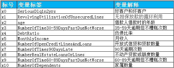
Figure 2-1 variables of original data
3, Data preprocessing
Before data processing, it is necessary to understand the missing value and abnormal value of data. Python has the describe() function, which can understand the missing value, mean and median of the data set.
    data = pd.read_csv('cs-training.csv')

    data.describe().to_csv('DataDescribe.csv')
Details of the dataset:

Figure 3-1 variable details
It can be seen from the above figure that the variables MonthlyIncome and NumberOfDependents are missing. The variable MonthlyIncome has 29731 missing values and NumberOfDependents has 3924 missing values.
3.1 missing value handling
This situation is very common in practical problems, which will lead to the unavailability of some analysis methods that can not deal with missing values. Therefore, we need to deal with missing values in the first step of credit risk rating model development. Missing value processing methods include the following.
(1) Directly delete samples with missing values.
(2) Missing values are filled according to the similarity between samples.
(3) Fill in the missing values according to the correlation between variables.
The missing rate of the variable MonthlyIncome is relatively large, so we fill in the missing value according to the correlation between variables. We use the random forest method:
def set_missing(df):

    process_df = df.ix[:,[5,0,1,2,3,4,6,7,8,9]]

    known = process_df[process_df.MonthlyIncome.notnull()].as_matrix()
    unknown = process_df[process_df.MonthlyIncome.isnull()].as_matrix()

    X = known[:, 1:]

    y = known[:, 0]

    rfr = RandomForestRegressor(random_state=0,
    n_estimators=200,max_depth=3,n_jobs=-1)
    rfr.fit(X,y)

    predicted = rfr.predict(unknown[:, 1:]).round(0)
    print(predicted)

    df.loc[(df.MonthlyIncome.isnull()), 'MonthlyIncome'] = predicted
    return df
The missing values of the NumberOfDependents variable are relatively few, and direct deletion will not have much impact on the overall model. After processing the missing values, delete the duplicates.
    data=set_missing(data)
    data=data.dropna()
    data = data.drop_duplicates()
    data.to_csv('MissingData.csv',index=False)
3.2 abnormal value handling
After the missing value is processed, we also need to process the abnormal value. Outliers refer to values that deviate significantly from most of the sampling data. For example, when the age of an individual customer is 0, it is generally considered as outliers. Outlier detection is usually used to find out the outliers in the sample population.
First, we find that there is 0 in the variable age, which is obviously an abnormal value. It is directly eliminated:
data = data[data['age'] > 0]
For the variables NumberOfTime30-59DaysPastDueNotWorse, NumberOfTimes90DaysLate and NumberOfTime60-89DaysPastDueNotWorse, it can be seen from the box diagram figure 3-2 below that there are abnormal values, and the unique function can know that there are 96 and 98 abnormal values, so they are eliminated. At the same time, it will be found that if the 96 and 98 values of one variable are eliminated, the 96 and 98 values of other variables will be eliminated accordingly.
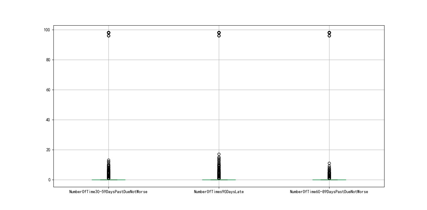
Figure 3-2 box diagram
The outliers of the variables numberoftime30-59dayspastduenotword, NumberOfTimes90DaysLate, numberoftime60-89dayspastduenotword are eliminated. In addition, in the data set, the good customer is 0 and the defaulting customer is 1. Considering the normal understanding, the customer who can perform the contract normally and pay interest is 1, so we take it inversely.
    data = data[data['NumberOfTime30-59DaysPastDueNotWorse'] < 90]

    data['SeriousDlqin2yrs']=1-data['SeriousDlqin2yrs']
3.3 data segmentation
In order to verify the fitting effect of the model, we need to segment the data set into training set and test set.
from sklearn.cross_validation import train_test_split
    Y = data['SeriousDlqin2yrs']
    X = data.ix[:, 1:]

    X_train, X_test, Y_train, Y_test = train_test_split(X, Y, test_size=0.3, random_state=0)

    train = pd.concat([Y_train, X_train], axis=1)
    test = pd.concat([Y_test, X_test], axis=1)
    clasTest = test.groupby('SeriousDlqin2yrs')['SeriousDlqin2yrs'].count()
    train.to_csv('TrainData.csv',index=False)
    test.to_csv('TestData.csv',index=False)
4, Exploratory analysis
Before establishing the model, we generally conduct Exploratory Data Analysis on the existing data. EDA refers to the exploration of existing data (especially the original data from investigation or observation) under as few a priori assumptions as possible. The commonly used Exploratory Data Analysis methods include histogram, scatter diagram and box diagram.
The age distribution of customers is shown in Figure 4-1. It can be seen that the age variable is roughly normally distributed, which is in line with the assumptions of statistical analysis.
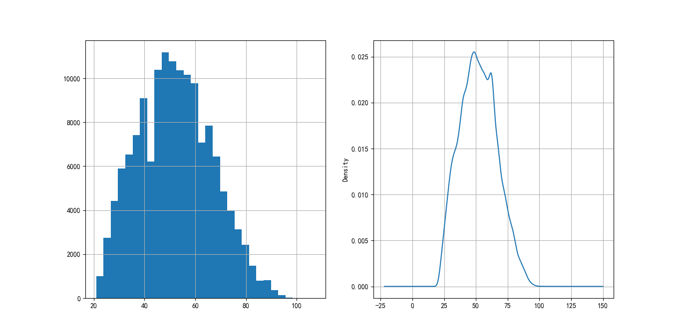
Figure 4-1 age distribution of customers
The annual income distribution of customers is shown in Figure 4-2, and the monthly income is also roughly normal distribution, which meets the needs of statistical analysis.
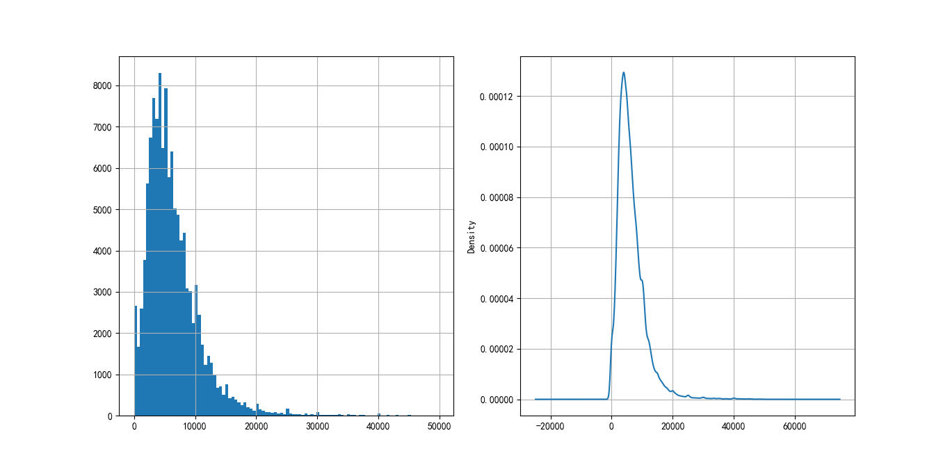
Figure 4-2 customer revenue distribution
5, Variable selection
Feature variable selection (ranking) is very important for data analysis and machine learning practitioners. Good feature selection can not only improve the performance of the model, but also help us understand the characteristics and underlying structure of the data, which plays an important role in further improving the model and algorithm. As for the variable selection code implementation of Python, you can refer to Combined with scikit learn, this paper introduces several common feature selection methods.
In this paper, we use the variable selection method of the credit scoring model, and use the WOE analysis method to determine whether the index meets the economic significance by comparing the default probability of the index box and the corresponding box. First, we discretize the variables.
5.1 sub box handling
Binning is a term for discretization of continuous variables. In the development of credit scoring card, there are commonly used isometric segmentation, equal depth segmentation and optimal segmentation. Among them, equidistant length intervals means that the intervals of segments are consistent, for example, the age takes ten years as a segment; Equal frequency intervals is to determine the number of segments first, and then make the number of data in each segment approximately equal; Optimal Binning, also known as supervised discretization, uses Recursive Partitioning to divide continuous variables into segments. Behind it is an algorithm to find better groups based on conditional inference.
Firstly, we choose the optimal segmentation of continuous variables. When the distribution of continuous variables does not meet the requirements of optimal segmentation, we consider equidistant segmentation of continuous variables. The code of the optimal bin division is as follows:
def mono_bin(Y, X, n = 20):
    r = 0
    good=Y.sum()
    bad=Y.count()-good
    while np.abs(r) < 1:
        d1 = pd.DataFrame({"X": X, "Y": Y, "Bucket": pd.qcut(X, n)})
        d2 = d1.groupby('Bucket', as_index = True)
        r, p = stats.spearmanr(d2.mean().X, d2.mean().Y)
        n = n - 1
    d3 = pd.DataFrame(d2.X.min(), columns = ['min'])
    d3['min']=d2.min().X
    d3['max'] = d2.max().X
    d3['sum'] = d2.sum().Y
    d3['total'] = d2.count().Y
    d3['rate'] = d2.mean().Y
    d3['woe']=np.log((d3['rate']/(1-d3['rate']))/(good/bad))
    d4 = (d3.sort_index(by = 'min')).reset_index(drop=True)
    print("=" * 60)
    print(d4)
    return d4
For, we will use optimal segmentation to classify the revolutionutilizationofunsecure lines, age, debt ratio and MonthlyIncome in the dataset.
Figure 5-1 box splitting of revolutionutilizationofunsecure lines.png
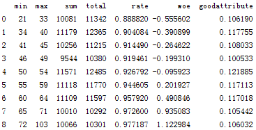
Figure 5-2 age distribution.png
Figure 5-3 DebtRatio box splitting.png
Figure 5-4 distribution of monthlyincome.png
For variables that cannot be optimally divided into boxes, the boxes are as follows:
    cutx3 = [ninf, 0, 1, 3, 5, pinf]
    cutx6 = [ninf, 1, 2, 3, 5, pinf]
    cutx7 = [ninf, 0, 1, 3, 5, pinf]
    cutx8 = [ninf, 0,1,2, 3, pinf]
    cutx9 = [ninf, 0, 1, 3, pinf]
    cutx10 = [ninf, 0, 1, 2, 3, 5, pinf]
5.2 WOE
WoE analysis is to divide the indicators, calculate the WoE value of each gear, and observe the change trend of WoE value with the indicators. The mathematical definition of WoE is:
woe=ln(goodattribute/badattribute)
During the analysis, we need to arrange each index from small to large, and calculate the WoE value of the corresponding grade. The larger the positive index, the smaller the WoE value; The larger the reverse index, the larger the WoE value. The greater the negative slope of the WoE value of the positive indicator and the greater the positive slope of the response indicator, it indicates that the indicator has good discrimination ability. If the WoE value approaches to a straight line, it means that the judgment ability of the index is weak. If there is a positive correlation trend between positive indicators and WoE and a negative correlation trend between negative indicators and WoE, it indicates that this indicator does not meet the economic significance and should be removed.
The woe function is implemented in mono in the previous section_ The bin() function already contains, which will not be repeated here.
5.3 correlation analysis and IV screening
Next, we will use the cleaned data to see the correlation between variables. Note that the correlation analysis here is only a preliminary check, and further check the VI (evidence weight) of the model as the basis for variable screening.
We call the heatmap() drawing function to draw the correlation diagram through the seaborn package in Python. The implementation code is as follows:
    corr = data.corr()
    xticks = ['x0','x1','x2','x3','x4','x5','x6','x7','x8','x9','x10']
    yticks = list(corr.index)
    fig = plt.figure()
    ax1 = fig.add_subplot(1, 1, 1)
    sns.heatmap(corr, annot=True, cmap='rainbow', ax=ax1, annot_kws={'size': 9, 'weight': 'bold', 'color': 'blue'})
    ax1.set_xticklabels(xticks, rotation=0, fontsize=10)
    ax1.set_yticklabels(yticks, rotation=0, fontsize=10)
    plt.show()
The generated graph is shown in Figure 5-5:
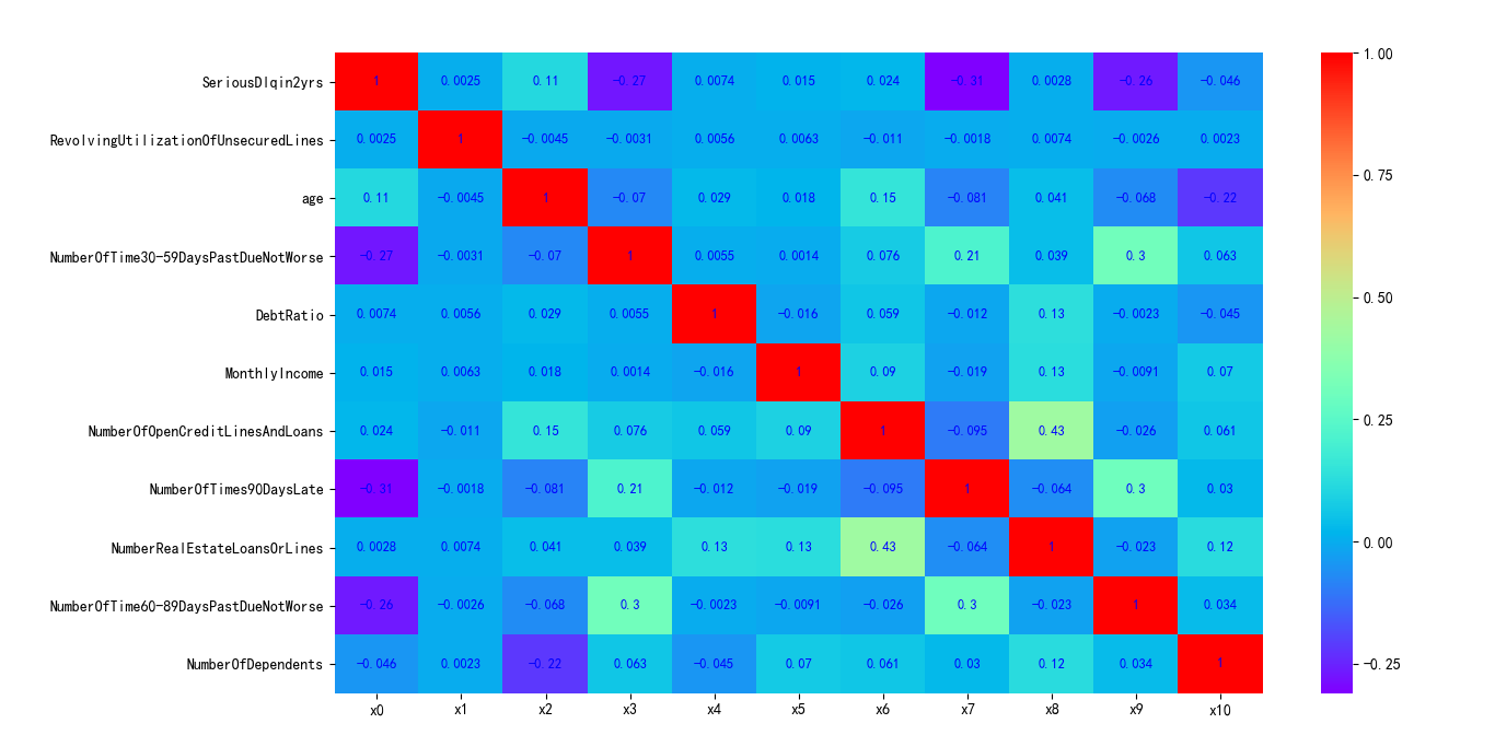
Figure 5-5 correlation of variables in data set
As can be seen from the above figure, the correlation between variables is very small. The correlation coefficient between NumberOfOpenCreditLinesAndLoans and NumberRealEstateLoansOrLines is 0.43.
Next, I further calculate the Infomation Value (IV) for each variable. IV index is generally used to determine the predictive ability of independent variables. The formula is:
IV=sum((goodattribute-badattribute)*ln(goodattribute/badattribute))
The criteria for judging the predictive ability of variables through IV value are:
< 0.02: unpredictive
0.02 to 0.1: weak
0.1 to 0.3: medium
0.3 to 0.5: strong
> 0.5: suspicious
IV Implementation in mono_ In the bin() function, the code is implemented as follows:
def mono_bin(Y, X, n = 20):
    r = 0
    good=Y.sum()
    bad=Y.count()-good
    while np.abs(r) < 1:
        d1 = pd.DataFrame({"X": X, "Y": Y, "Bucket": pd.qcut(X, n)})
        d2 = d1.groupby('Bucket', as_index = True)
        r, p = stats.spearmanr(d2.mean().X, d2.mean().Y)
        n = n - 1
    d3 = pd.DataFrame(d2.X.min(), columns = ['min'])
    d3['min']=d2.min().X
    d3['max'] = d2.max().X
    d3['sum'] = d2.sum().Y
    d3['total'] = d2.count().Y
    d3['rate'] = d2.mean().Y
    d3['woe']=np.log((d3['rate']/(1-d3['rate']))/(good/bad))
    d3['goodattribute']=d3['sum']/good
    d3['badattribute']=(d3['total']-d3['sum'])/bad
    iv=((d3['goodattribute']-d3['badattribute'])*d3['woe']).sum()
    d4 = (d3.sort_index(by = 'min')).reset_index(drop=True)
    print("=" * 60)
    print(d4)
    cut=[]
    cut.append(float('-inf'))
    for i in range(1,n+1):
        qua=X.quantile(i/(n+1))
        cut.append(round(qua,4))
    cut.append(float('inf'))
    woe=list(d4['woe'].round(3))
    return d4,iv,cut,woe
Generated IV diagram Code:
    ivlist=[ivx1,ivx2,ivx3,ivx4,ivx5,ivx6,ivx7,ivx8,ivx9,ivx10]
    index=['x1','x2','x3','x4','x5','x6','x7','x8','x9','x10']
    fig1 = plt.figure(1)
    ax1 = fig1.add_subplot(1, 1, 1)
    x = np.arange(len(index))+1
    ax1.bar(x, ivlist, width=0.4)
    ax1.set_xticks(x)
    ax1.set_xticklabels(index, rotation=0, fontsize=12)
    ax1.set_ylabel('IV(Information Value)', fontsize=14)

    for a, b in zip(x, ivlist):
        plt.text(a, b + 0.01, '%.4f' % b, ha='center', va='bottom', fontsize=10)
    plt.show()
Output image:
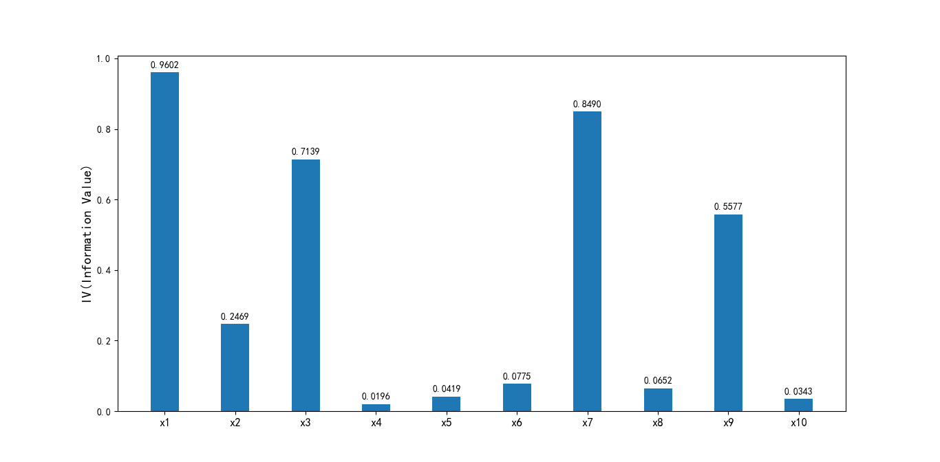
Figure 5-6 IV diagram of output variables
It can be seen that the IV values of the DebtRatio, MonthlyIncome, NumberOfOpenCreditLinesAndLoans, NumberRealEstateLoansOrLines and NumberOfDependents variables are obviously low, so they are deleted.
Summary
This paper mainly introduces the data preprocessing, exploratory analysis and variable selection in the development of credit scoring model. Data preprocessing mainly uses random forest method and direct elimination method to deal with missing values. For outliers, outliers are eliminated mainly according to the actual situation and the data distribution of box chart; Exploratory analysis mainly makes an initial inquiry into the distribution of each variable; Variable selection mainly considers the box division method of variables, calculates the WOE value according to the box division results, then checks the correlation between variables, and selects the variables with good effect on data processing according to the IV value of each variable.
. Next, we will continue to discuss the model implementation and analysis of credit scoring card, credit scoring method and automatic scoring system.
6, Model analysis
Weight of evidence (WOE) transformation can transform Logistic regression model into standard scorecard format. The purpose of introducing WOE conversion is not to improve the quality of the model, but some variables should not be included in the model, either because they can not increase the model value, or because the error related to its model correlation coefficient is large. In fact, WOE conversion can not be used to establish a standard credit scoring card. In this case, the Logistic regression model needs to deal with a larger number of independent variables. Although this will increase the complexity of the modeling program, the final score cards are the same.
Before establishing the model, we need to convert the filtered variables into WoE values for credit scoring.
6.1 WOE conversion
We have obtained the box data and woe data of each variable. We only need to replace them according to the variable data. The implementation code is as follows:
def replace_woe(series,cut,woe):
    list=[]
    i=0
    while i<len(series):
        value=series[i]
        j=len(cut)-2
        m=len(cut)-2
        while j>=0:
            if value>=cut[j]:
                j=-1
            else:
                j -=1
                m -= 1
        list.append(woe[m])
        i += 1
    return list
We replace each variable and save it in the WoeData.csv file:
    data['RevolvingUtilizationOfUnsecuredLines'] = Series(replace_woe(data['RevolvingUtilizationOfUnsecuredLines'], cutx1, woex1))
    data['age'] = Series(replace_woe(data['age'], cutx2, woex2))
    data['NumberOfTime30-59DaysPastDueNotWorse'] = Series(replace_woe(data['NumberOfTime30-59DaysPastDueNotWorse'], cutx3, woex3))
    data['DebtRatio'] = Series(replace_woe(data['DebtRatio'], cutx4, woex4))
    data['MonthlyIncome'] = Series(replace_woe(data['MonthlyIncome'], cutx5, woex5))
    data['NumberOfOpenCreditLinesAndLoans'] = Series(replace_woe(data['NumberOfOpenCreditLinesAndLoans'], cutx6, woex6))
    data['NumberOfTimes90DaysLate'] = Series(replace_woe(data['NumberOfTimes90DaysLate'], cutx7, woex7))
    data['NumberRealEstateLoansOrLines'] = Series(replace_woe(data['NumberRealEstateLoansOrLines'], cutx8, woex8))
    data['NumberOfTime60-89DaysPastDueNotWorse'] = Series(replace_woe(data['NumberOfTime60-89DaysPastDueNotWorse'], cutx9, woex9))
    data['NumberOfDependents'] = Series(replace_woe(data['NumberOfDependents'], cutx10, woex10))
    data.to_csv('WoeData.csv', index=False)
6.2 establishment of logic model
We directly call the statsmodels package to implement logical regression:
    Import data
    data = pd.read_csv('WoeData.csv')

    Y=data['SeriousDlqin2yrs']

    X=data.drop(['SeriousDlqin2yrs','DebtRatio','MonthlyIncome', 'NumberOfOpenCreditLinesAndLoans','NumberRealEstateLoansOrLines','NumberOfDependents'],axis=1)
    X1=sm.add_constant(X)
    logit=sm.Logit(Y,X1)
    result=logit.fit()
    print(result.summary())
Output results:

Figure 6-1 results of logistic regression model.png
It can be seen from figure 6-1 that all variables of logistic regression have passed the significance test and meet the requirements.
6.3 model inspection
Here, our modeling part is basically over. We need to verify the prediction ability of the model. We use the test data reserved at the beginning of modeling for verification. The fitting ability of the model was evaluated by ROC curve and AUC.
In Python, you can use sklearn.metrics, which can easily compare two classifiers and automatically calculate ROC and AUC.
Implementation code:
    Y_test = test['SeriousDlqin2yrs']

    X_test = test.drop(['SeriousDlqin2yrs', 'DebtRatio', 'MonthlyIncome', 'NumberOfOpenCreditLinesAndLoans','NumberRealEstateLoansOrLines', 'NumberOfDependents'], axis=1)
    X3 = sm.add_constant(X_test)
    resu = result.predict(X3)
    fpr, tpr, threshold = roc_curve(Y_test, resu)
    rocauc = auc(fpr, tpr)
    plt.plot(fpr, tpr, 'b', label='AUC = %0.2f' % rocauc)
    plt.legend(loc='lower right')
    plt.plot([0, 1], [0, 1], 'r--')
    plt.xlim([0, 1])
    plt.ylim([0, 1])
    plt.ylabel('Real rate')
    plt.xlabel('False positive rate')
    plt.show()
Output results:
It can be seen from the above figure that the AUC value is 0.85, indicating that the prediction effect of the model is good and the accuracy is high.
7, Credit score
We have basically completed the work related to modeling, and verified the prediction ability of the model with ROC curve. The next step is to convert the Logistic model into a standard scorecard.
7.1 scoring criteria
According to the above paper data:
a=log(p_good/P_bad)
Score = offset + factor * log(odds)
Before establishing a standard scorecard, we need to select several scorecard parameters: basic score, PDO (score of doubling ratio) and good / bad ratio. Here, we take 600 as the basic score, the PDO is 20 (double the good / bad ratio for every 20 points higher), and the good / bad ratio is 20.
    p = 20 / math.log(2)
    q = 600 - 20 * math.log(20) / math.log(2)
    baseScore = round(q + p * coe[0], 0)
Individual total score = basic score + scores of each part
7.2 partial score
Next, calculate the score of each variable part. Score function of each part:
def get_score(coe,woe,factor):
    scores=[]
    for w in woe:
        score=round(coe*w*factor,0)
        scores.append(score)
    return scores
Calculate the score of each variable:
    x1 = get_score(coe[1], woex1, p)
    x2 = get_score(coe[2], woex2, p)
    x3 = get_score(coe[3], woex3, p)
    x7 = get_score(coe[4], woex7, p)
    x9 = get_score(coe[5], woex9, p)
We can get the score card of each part, as shown in Figure 7-1:
8, Automatic scoring system
The score is calculated according to the variable as follows:
def compute_score(series,cut,score):
    list = []
    i = 0
    while i < len(series):
        value = series[i]
        j = len(cut) - 2
        m = len(cut) - 2
        while j >= 0:
            if value >= cut[j]:
                j = -1
            else:
                j -= 1
                m -= 1
        list.append(score[m])
        i += 1
    return list
Let's calculate the score in test:
    test1 = pd.read_csv('TestData.csv')
    test1['BaseScore']=Series(np.zeros(len(test1)))+baseScore
    test1['x1'] = Series(compute_score(test1['RevolvingUtilizationOfUnsecuredLines'], cutx1, x1))
    test1['x2'] = Series(compute_score(test1['age'], cutx2, x2))
    test1['x3'] = Series(compute_score(test1['NumberOfTime30-59DaysPastDueNotWorse'], cutx3, x3))
    test1['x7'] = Series(compute_score(test1['NumberOfTimes90DaysLate'], cutx7, x7))
    test1['x9'] = Series(compute_score(test1['NumberOfTime60-89DaysPastDueNotWorse'], cutx9, x9))
    test1['Score'] = test1['x1'] + test1['x2'] + test1['x3'] + test1['x7'] +test1['x9']  + baseScore
    test1.to_csv('ScoreData.csv', index=False)
Partial results of batch calculation:
9, Summary and Prospect
In this paper, through the analysis of Give Me Some Credit Data mining and analysis, combined with the establishment principle of credit scoring card, from data preprocessing, variable selection, modeling and analysis to creating credit scoring, a simple credit scoring system is created.
The AI based machine learning scorecard system can make the system more powerful by eliminating the old data (after a certain time point, such as 2 years), then automatically modeling, model evaluation, and continuously optimizing the characteristic variables.
summary
The main process of Python based credit scorecard model is introduced here, but there are many details in the actual scorecard modeling, which are described too hastily or even incorrectly on the Internet. For example, if the missing rate of a variable reaches 80% - 90%, should the variable be deleted directly? Can the correlation of variables as high as 0.8 be removed? Experienced modelers need to find a balance between mathematical theory, actual needs of business lines, computer test results and other aspects, rather than thinking from one perspective. It's like experienced surgeons don't necessarily follow textbook theories. There are many disputes in the fields of statistics, machine learning, artificial intelligence and so on. You should maintain the ability of independent thinking when studying, so as to continuously optimize the data and scientific knowledge.
Python based credit card model - give me some credit is introduced here. Welcome to sign up< python financial risk control scorecard model and data analysis micro professional course>
https://edu.csdn.net/combo/detail/1927
Learn more about it.
Code network disk address
Baidu online disk download link: https://pan.baidu.com/s/14xMcCRSvnjrwhM7t6ZEOgw
Extraction code: 1234
reference
python financial risk control scorecard model and data analysis
Modeling and analysis of credit scoring card based on R language
Credit card scoring model
Development and implementation of credit standard score card model
Teach you how to build a credit scoring model in R language
Scorecard Model
Data cleaning using python
Monotonic Binning with Python
Python outlier handling and detection
Combined with scikit learn, this paper introduces several common feature selection methods
Analysis of credit scoring card model based on Python