1. math function
1.1 special constant
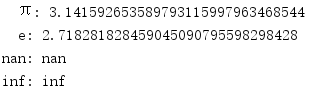
Many mathematical operations depend on special constants. math contains values of π (pi), e, Nan (not a number) and infinity (infinity).
import math

print('  π: {:.30f}'.format(math.pi))
print('  e: {:.30f}'.format(math.e))
print('nan: {:.30f}'.format(math.nan))
print('inf: {:.30f}'.format(math.inf))
The precision of π and e is only limited by the floating point C library of the platform.
1.2 test outliers
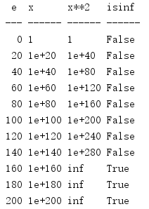
Floating point calculations can cause two types of outliers. The first is inf (infinite). When double is used to store a floating-point number, and the value overflows from a specific large absolute value, the exception value will appear.
import math

print('{:^3} {:6} {:6} {:6}'.format(
    'e', 'x', 'x**2', 'isinf'))
print('{:-^3} {:-^6} {:-^6} {:-^6}'.format(
    '', '', '', ''))

for e in range(0, 201, 20):
    x = 10.0 ** e
    y = x * x
    print('{:3d} {:<6g} {:<6g} {!s:6}'.format(
        e, x, y, math.isinf(y),
    ))
When the exponent in this example becomes large enough, the square of x cannot be stored in another double, and this value will be recorded as infinite.
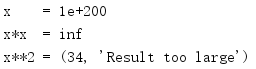
However, not all floating-point overflows result in inf values. Specifically, when calculating an exponent with a floating-point value, an overflow error is generated instead of retaining the inf result.
x = 10.0 ** 200

print('x    =', x)
print('x*x  =', x * x)
print('x**2 =', end=' ')
try:
    print(x ** 2)
except OverflowError as err:
    print(err)
This difference is due to implementation differences in the libraries used by C and Python.
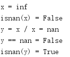
Division operation with infinite value is undefined. The result of dividing a number by an infinite value is Nan (not a number).
import math

x = (10.0 ** 200) * (10.0 ** 200)
y = x / x

print('x =', x)
print('isnan(x) =', math.isnan(x))
print('y = x / x =', x / x)
print('y == nan =', y == float('nan'))
print('isnan(y) =', math.isnan(y))
nan is not equal to any value, or even itself, so to check nan, you need to use isnan().
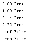
You can use isfinish () to check whether it is a normal number or a special value, inf or nan.
import math

for f in [0.0, 1.0, math.pi, math.e, math.inf, math.nan]:
    print('{:5.2f} {!s}'.format(f, math.isfinite(f)))
If it is a special value inf or nan, isfinish() returns false, otherwise it returns true.
1.3 comparison
When it comes to floating-point values, it's easy to make mistakes. Every step of calculation may introduce errors due to numerical representation. The isclose() function uses a stable algorithm to minimize these errors and complete relative and absolute comparisons. The formula used is equivalent to:
abs(a-b) <= max(rel_tol * max(abs(a), abs(b)), abs_tol)
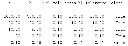
By default, isclose() completes the relative comparison and the tolerance is set to le-09, which means that the difference between the two values must be less than or equal to le times the larger absolute value in a and b. You can change this tolerance by passing the keyword parameter rel_tol to isclose(). In this case, the gap between values must be within 10%.
import math

INPUTS = [
    (1000, 900, 0.1),
    (100, 90, 0.1),
    (10, 9, 0.1),
    (1, 0.9, 0.1),
    (0.1, 0.09, 0.1),
]

print('{:^8} {:^8} {:^8} {:^8} {:^8} {:^8}'.format(
    'a', 'b', 'rel_tol', 'abs(a-b)', 'tolerance', 'close')
)
print('{:-^8} {:-^8} {:-^8} {:-^8} {:-^8} {:-^8}'.format(
    '-', '-', '-', '-', '-', '-'),
)

fmt = '{:8.2f} {:8.2f} {:8.2f} {:8.2f} {:8.2f} {!s:>8}'

for a, b, rel_tol in INPUTS:
    close = math.isclose(a, b, rel_tol=rel_tol)
    tolerance = rel_tol * max(abs(a), abs(b))
    abs_diff = abs(a - b)
    print(fmt.format(a, b, rel_tol, abs_diff, tolerance, close))
The comparison between 0.1 and 0.09 failed because the error represents 0.1.
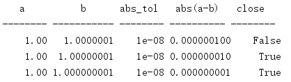
To use a fixed or "absolute" tolerance, you can pass in ABS? Tol instead of rel? Tol.
import math

INPUTS = [
    (1.0, 1.0 + 1e-07, 1e-08),
    (1.0, 1.0 + 1e-08, 1e-08),
    (1.0, 1.0 + 1e-09, 1e-08),
]

print('{:^8} {:^11} {:^8} {:^10} {:^8}'.format(
    'a', 'b', 'abs_tol', 'abs(a-b)', 'close')
)
print('{:-^8} {:-^11} {:-^8} {:-^10} {:-^8}'.format(
    '-', '-', '-', '-', '-'),
)

for a, b, abs_tol in INPUTS:
    close = math.isclose(a, b, abs_tol=abs_tol)
    abs_diff = abs(a - b)
    print('{:8.2f} {:11} {:8} {:0.9f} {!s:>8}'.format(
        a, b, abs_tol, abs_diff, close))
For absolute tolerance, the difference between the input values must be less than the given tolerance.
nan and inf are special cases.
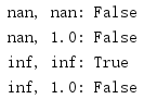
import math

print('nan, nan:', math.isclose(math.nan, math.nan))
print('nan, 1.0:', math.isclose(math.nan, 1.0))
print('inf, inf:', math.isclose(math.inf, math.inf))
print('inf, 1.0:', math.isclose(math.inf, 1.0))
nan is not close to any value, including itself. inf is only close to itself.
1.4 converting floating point values to integers
There are three functions in the math module to convert floating-point values to integers. These three functions adopt different methods and are suitable for different situations.
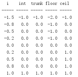
The simplest is trunc(), which truncates the number after the decimal point, leaving only the significant digits that make up the integral part of the value. floor() converts its input to no greater than its maximum integer, and ceil () (upper limit) generates the smallest integer in sequence after the input value.
import math

HEADINGS = ('i', 'int', 'trunk', 'floor', 'ceil')
print('{:^5} {:^5} {:^5} {:^5} {:^5}'.format(*HEADINGS))
print('{:-^5} {:-^5} {:-^5} {:-^5} {:-^5}'.format(
    '', '', '', '', '',
))

fmt = '{:5.1f} {:5.1f} {:5.1f} {:5.1f} {:5.1f}'

TEST_VALUES = [
    -1.5,
    -0.8,
    -0.5,
    -0.2,
    0,
    0.2,
    0.5,
    0.8,
    1,
]

for i in TEST_VALUES:
    print(fmt.format(
        i,
        int(i),
        math.trunc(i),
        math.floor(i),
        math.ceil(i),
    ))
trunc() is equivalent to a direct conversion to int.
1.5 other representations of floating point values
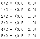
modf() takes a floating-point number and returns a tuple containing the decimal and integer parts of the input value.
import math

for i in range(6):
    print('{}/2 = {}'.format(i, math.modf(i / 2.0)))
Both numbers in the return value are floating-point numbers.
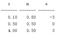
frexp() returns the mantissa and exponent of a floating-point number, which can be used to create a more portable representation of the value.
import math

print('{:^7} {:^7} {:^7}'.format('x', 'm', 'e'))
print('{:-^7} {:-^7} {:-^7}'.format('', '', ''))

for x in [0.1, 0.5, 4.0]:
    m, e = math.frexp(x)
    print('{:7.2f} {:7.2f} {:7d}'.format(x, m, e))
frexp() uses the formula x = m * 2**e and returns the values m and E.
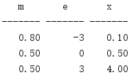
ldexp() is the opposite of frexp().
import math

print('{:^7} {:^7} {:^7}'.format('m', 'e', 'x'))
print('{:-^7} {:-^7} {:-^7}'.format('', '', ''))

INPUTS = [
    (0.8, -3),
    (0.5, 0),
    (0.5, 3),
]

for m, e in INPUTS:
    x = math.ldexp(m, e)
    print('{:7.2f} {:7d} {:7.2f}'.format(m, e, x))
ldexp() uses the same formula as frexp(), takes the mantissa and index values as parameters, and returns a floating-point number.
1.6 plus sign and minus sign
The absolute value of a number is its own value without a sign. fabs() can be used to calculate the absolute value of a floating-point number.
import math

print(math.fabs(-1.1))
print(math.fabs(-0.0))
print(math.fabs(0.0))
print(math.fabs(1.1))
In practice, the absolute value of float is expressed as a positive value.

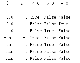
To determine the symbol of a value so that you can specify the same symbol for a group of values or compare two values, use copysign() to set the symbol of the correct value.
import math

HEADINGS = ('f', 's', '< 0', '> 0', '= 0')
print('{:^5} {:^5} {:^5} {:^5} {:^5}'.format(*HEADINGS))
print('{:-^5} {:-^5} {:-^5} {:-^5} {:-^5}'.format(
    '', '', '', '', '',
))

VALUES = [
    -1.0,
    0.0,
    1.0,
    float('-inf'),
    float('inf'),
    float('-nan'),
    float('nan'),
]

for f in VALUES:
    s = int(math.copysign(1, f))
    print('{:5.1f} {:5d} {!s:5} {!s:5} {!s:5}'.format(
        f, s, f < 0, f > 0, f == 0,
    ))
Another function similar to copysign() is also needed because nan and - nan cannot be compared directly with other values.
1.7 common calculation
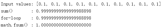
It is very difficult to express precision in binary floating-point memory. Some values cannot be expressed accurately, and if a value is processed by repeated calculation, the more frequent the calculation, the easier it is to introduce error. math contains a function to calculate the sum of a series of floating-point numbers. It uses an efficient algorithm to minimize this error.
import math

values = [0.1] * 10

print('Input values:', values)

print('sum()       : {:.20f}'.format(sum(values)))

s = 0.0
for i in values:
    s += i
print('for-loop    : {:.20f}'.format(s))

print('math.fsum() : {:.20f}'.format(math.fsum(values)))
Given a sequence of 10 values, each of which is equal to 0.1, the expected sum of the sequences is 1.0. However, since 0.1 cannot be represented exactly as a floating-point number, an error is introduced into the sum, unless it is calculated with fsum().
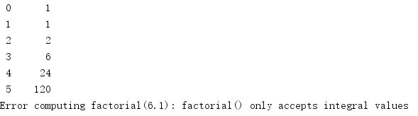
factorial() is often used to calculate the number of permutations and combinations of a series of objects. The factorial (expressed as n!) of a positive integer n is defined as (n-1)!*n recursively, and recursion stops at 0! = = 1.
import math

for i in [0, 1.0, 2.0, 3.0, 4.0, 5.0, 6.1]:
    try:
        print('{:2.0f} {:6.0f}'.format(i, math.factorial(i)))
    except ValueError as err:
        print('Error computing factorial({}): {}'.format(i, err))
factorial() can only handle integers, but it does accept the float parameter as long as it can be converted to an integer without losing value.
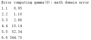
gamma() is similar to factorial(), but it can handle real numbers, and the value moves down a number (gamma equals (n - 1)!).
import math

for i in [0, 1.1, 2.2, 3.3, 4.4, 5.5, 6.6]:
    try:
        print('{:2.1f} {:6.2f}'.format(i, math.gamma(i)))
    except ValueError as err:
        print('Error computing gamma({}): {}'.format(i, err))
This is not allowed because 0 causes the start value to be negative.
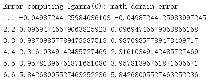
lgamma() returns the natural logarithm of the absolute value of the result obtained by gamma on the input value.
import math

for i in [0, 1.1, 2.2, 3.3, 4.4, 5.5, 6.6]:
    try:
        print('{:2.1f} {:.20f} {:.20f}'.format(
            i,
            math.lgamma(i),
            math.log(math.gamma(i)),
        ))
    except ValueError as err:
        print('Error computing lgamma({}): {}'.format(i, err))
Using lgamma() is more accurate than using gamma() results to calculate the logarithm alone.
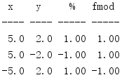
The modulus (%) operator calculates the remainder of a division expression (for example, 5% 2 = 1). The built-in operator in Python can handle integers well, but like many other floating-point operations, the intermediate calculation may cause representation problems and further data loss. fmod() can provide a more precise implementation for floating-point values.
import math

print('{:^4} {:^4} {:^5} {:^5}'.format(
    'x', 'y', '%', 'fmod'))
print('{:-^4} {:-^4} {:-^5} {:-^5}'.format(
    '-', '-', '-', '-'))

INPUTS = [
    (5, 2),
    (5, -2),
    (-5, 2),
]

for x, y in INPUTS:
    print('{:4.1f} {:4.1f} {:5.2f} {:5.2f}'.format(
        x,
        y,
        x % y,
        math.fmod(x, y),
    ))
There may also be confusion, that is, the algorithm used by fmod() is different from that used by% so the symbol of the result is different.
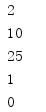
You can use gcd() to find the largest integer of two integer common divisors - that is, the largest common divisor.
import math

print(math.gcd(10, 8))
print(math.gcd(10, 0))
print(math.gcd(50, 225))
print(math.gcd(11, 9))
print(math.gcd(0, 0))
If both values are 0, the result is 0.
1.8 index and logarithm
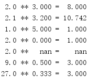
Exponential growth curves often appear in economics, physics and other sciences. Python has a built-in power operator ("* *"), but if you need to use a callable function as an argument to another function, you may need to use pow().
import math

INPUTS = [
    # Typical uses
    (2, 3),
    (2.1, 3.2),

    # Always 1
    (1.0, 5),
    (2.0, 0),

    # Not-a-number
    (2, float('nan')),

    # Roots
    (9.0, 0.5),
    (27.0, 1.0 / 3),
]

for x, y in INPUTS:
    print('{:5.1f} ** {:5.3f} = {:6.3f}'.format(
        x, y, math.pow(x, y)))
Any power of 1 always returns 1.0. Similarly, when the exponent of any value is 0.0, it always returns 1.0. For nan value (not a number), most operations return nan. If the index is less than 1, pow() calculates a root.
Because the square root (exponential 1 / 2) is used very frequently, there is a separate function to calculate the square root.
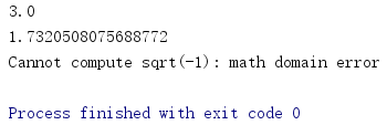
import math

print(math.sqrt(9.0))
print(math.sqrt(3))
try:
    print(math.sqrt(-1))
except ValueError as err:
    print('Cannot compute sqrt(-1):', err)
Complex numbers are required to calculate the square root of a negative number, which is outside the scope of math. An attempt to calculate the square root of a negative value results in a ValueError.
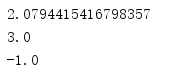
The logarithmic function looks for y satisfying the condition x=b**y. The default log() calculates the natural logarithm (the base is e). If a second parameter is provided, the parameter value is used as the base.
import math

print(math.log(8))
print(math.log(8, 2))
print(math.log(0.5, 2))
When x is less than 1, the logarithm will produce a negative result.
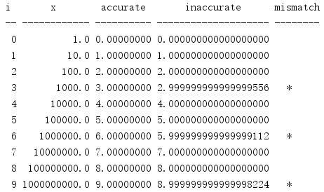
log() has three variants. Given the representation and rounding errors of floating-point numbers, the calculated values generated by log(x,b) have only limited precision (especially for some base numbers). log10() completes the log(x,10) calculation, but uses a more precise algorithm than log().
import math

print('{:2} {:^12} {:^10} {:^20} {:8}'.format(
    'i', 'x', 'accurate', 'inaccurate', 'mismatch',
))
print('{:-^2} {:-^12} {:-^10} {:-^20} {:-^8}'.format(
    '', '', '', '', '',
))

for i in range(0, 10):
    x = math.pow(10, i)
    accurate = math.log10(x)
    inaccurate = math.log(x, 10)
    match = '' if int(inaccurate) == i else '*'
    print('{:2d} {:12.1f} {:10.8f} {:20.18f} {:^5}'.format(
        i, x, accurate, inaccurate, match,
    ))
Lines with * at the end of the output highlight imprecise values.
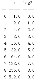
Similar to log10(), log2() will complete the calculation equivalent to math.log(x,2).
import math

print('{:>2} {:^5} {:^5}'.format(
    'i', 'x', 'log2',
))
print('{:-^2} {:-^5} {:-^5}'.format(
    '', '', '',
))

for i in range(0, 10):
    x = math.pow(2, i)
    result = math.log2(x)
    print('{:2d} {:5.1f} {:5.1f}'.format(
        i, x, result,
    ))
Depending on the underlying platform, this built-in special-purpose function provides better performance and precision because it utilizes special-purpose algorithms for base 2, which are not used in more general-purpose functions.
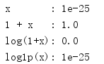
log1p() computes the Newton Mercator sequence (natural logarithm of 1+x).
import math

x = 0.0000000000000000000000001
print('x       :', x)
print('1 + x   :', 1 + x)
print('log(1+x):', math.log(1 + x))
print('log1p(x):', math.log1p(x))
For x close to 0, log1p() is more accurate because it uses an algorithm that compensates for rounding errors caused by the initial addition.
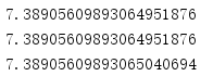
exp() calculates the exponential function (e**x).
import math

x = 2

fmt = '{:.20f}'
print(fmt.format(math.e ** 2))
print(fmt.format(math.pow(math.e, 2)))
print(fmt.format(math.exp(2)))
Similar to other special functions, the algorithm used by exp() can generate more accurate results than the equivalent general function, math.pow(math.e,x).
expm1() is the inverse operation of log1p(), accounting for e**x-1.
import math

x = 0.0000000000000000000000001

print(x)
print(math.exp(x) - 1)
print(math.expm1(x))
Similar to log1p(), the value of x is very small. If the subtraction is completed separately, the accuracy may be lost.

1.9 corners
Although we often talk about angles in degrees every day, radians are the standard unit for measuring angles in science and mathematics. Radian is the angle formed by two lines intersecting at the center of a circle. Its end point falls on the circumference of the circle, and the distance between the end points is one radian.
The circle length is calculated as 2 π r, so there is a relationship between the radian and π (this is a value often used in trigonometric function calculation). This relationship makes the use of radians in trigonometry and calculus, because more compact formulas can be obtained by using radians.
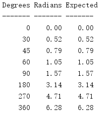
To convert degrees to radians, use redians().
import math

print('{:^7} {:^7} {:^7}'.format(
    'Degrees', 'Radians', 'Expected'))
print('{:-^7} {:-^7} {:-^7}'.format(
    '', '', ''))

INPUTS = [
    (0, 0),
    (30, math.pi / 6),
    (45, math.pi / 4),
    (60, math.pi / 3),
    (90, math.pi / 2),
    (180, math.pi),
    (270, 3 / 2.0 * math.pi),
    (360, 2 * math.pi),
]

for deg, expected in INPUTS:
    print('{:7d} {:7.2f} {:7.2f}'.format(
        deg,
        math.radians(deg),
        expected,
    ))
The conversion formula is rad = deg * π / 180.
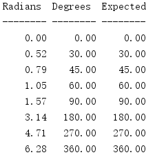
To convert from radians to degrees, use degrees().
import math

INPUTS = [
    (0, 0),
    (math.pi / 6, 30),
    (math.pi / 4, 45),
    (math.pi / 3, 60),
    (math.pi / 2, 90),
    (math.pi, 180),
    (3 * math.pi / 2, 270),
    (2 * math.pi, 360),
]

print('{:^8} {:^8} {:^8}'.format(
    'Radians', 'Degrees', 'Expected'))
print('{:-^8} {:-^8} {:-^8}'.format('', '', ''))
for rad, expected in INPUTS:
    print('{:8.2f} {:8.2f} {:8.2f}'.format(
        rad,
        math.degrees(rad),
        expected,
    ))
The specific conversion formula is deg = rad * 180 / π.
1.10 trigonometric function
Trigonometric functions associate the angle in a triangle with its edge length. Trigonometric functions are often used in formulas with periodic properties, such as harmonic or circular motion; trigonometric functions are also often used in dealing with angles. The angle parameters of all trigonometric functions in the standard library are expressed as radians.
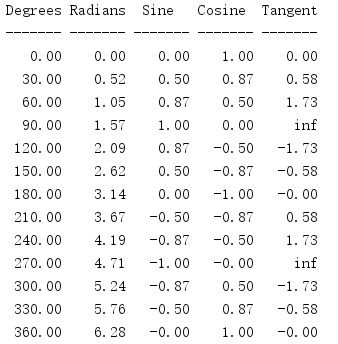
Given an angle in a right triangle, its sine is the ratio of the length of the opposite side to the length of the hypotenuse (sin A = opposite side / hypotenuse). Cosine is the ratio of the length of the adjacent edge to the length of the hypotenuse (cos A = adjacent / hypotenuse). Tangent is the ratio of opposite side to adjacent side (tan A = opposite side / adjacent side).
import math

print('{:^7} {:^7} {:^7} {:^7} {:^7}'.format(
    'Degrees', 'Radians', 'Sine', 'Cosine', 'Tangent'))
print('{:-^7} {:-^7} {:-^7} {:-^7} {:-^7}'.format(
    '-', '-', '-', '-', '-'))

fmt = '{:7.2f} {:7.2f} {:7.2f} {:7.2f} {:7.2f}'

for deg in range(0, 361, 30):
    rad = math.radians(deg)
    if deg in (90, 270):
        t = float('inf')
    else:
        t = math.tan(rad)
    print(fmt.format(deg, rad, math.sin(rad), math.cos(rad), t))
Tangent can also be defined as the ratio of the sine value of the angle to its cosine value. Because the cosine of radians π / 2 and 3 π / 2 is 0, the corresponding tangent value is infinite.
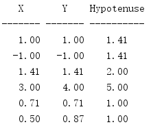
Given a point (x,y), point [(0,0),(x,0),(x,y)], the length of the hypotenuse in the triangle is (x**2+y**2)**1/2, which can be calculated by hypot().
import math

print('{:^7} {:^7} {:^10}'.format('X', 'Y', 'Hypotenuse'))
print('{:-^7} {:-^7} {:-^10}'.format('', '', ''))

POINTS = [
    # simple points
    (1, 1),
    (-1, -1),
    (math.sqrt(2), math.sqrt(2)),
    (3, 4),  # 3-4-5 triangle
    # on the circle
    (math.sqrt(2) / 2, math.sqrt(2) / 2),  # pi/4 rads
    (0.5, math.sqrt(3) / 2),  # pi/3 rads
]

for x, y in POINTS:
    h = math.hypot(x, y)
    print('{:7.2f} {:7.2f} {:7.2f}'.format(x, y, h))
For a point on a circle, its hypotenuse is always equal to 1.
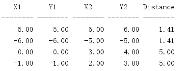
You can also use this function to see the distance between two points.
import math

print('{:^8} {:^8} {:^8} {:^8} {:^8}'.format(
    'X1', 'Y1', 'X2', 'Y2', 'Distance',
))
print('{:-^8} {:-^8} {:-^8} {:-^8} {:-^8}'.format(
    '', '', '', '', '',
))

POINTS = [
    ((5, 5), (6, 6)),
    ((-6, -6), (-5, -5)),
    ((0, 0), (3, 4)),  # 3-4-5 triangle
    ((-1, -1), (2, 3)),  # 3-4-5 triangle
]

for (x1, y1), (x2, y2) in POINTS:
    x = x1 - x2
    y = y1 - y2
    h = math.hypot(x, y)
    print('{:8.2f} {:8.2f} {:8.2f} {:8.2f} {:8.2f}'.format(
        x1, y1, x2, y2, h,
    ))
Use the difference between the x value and the y value to move an endpoint to the origin, and pass the result in hypot().
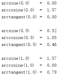
math also defines anti trigonometric functions.
import math

for r in [0, 0.5, 1]:
    print('arcsine({:.1f})    = {:5.2f}'.format(r, math.asin(r)))
    print('arccosine({:.1f})  = {:5.2f}'.format(r, math.acos(r)))
    print('arctangent({:.1f}) = {:5.2f}'.format(r, math.atan(r)))
    print()
1.57 for π / 2, or 90 degrees, the sine of this angle is 1 and the cosine is 0.
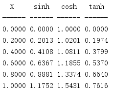
1.11 hyperbolic function
Hyperbolic functions are often used in linear differential equations to deal with electromagnetic field, fluid mechanics, special relativity and other advanced physical and mathematical problems.
import math

print('{:^6} {:^6} {:^6} {:^6}'.format(
    'X', 'sinh', 'cosh', 'tanh',
))
print('{:-^6} {:-^6} {:-^6} {:-^6}'.format('', '', '', ''))

fmt = '{:6.4f} {:6.4f} {:6.4f} {:6.4f}'

for i in range(0, 11, 2):
    x = i / 10.0
    print(fmt.format(
        x,
        math.sinh(x),
        math.cosh(x),
        math.tanh(x),
    ))
Cosine function and sine function form a circle, while hyperbolic cosine function and hyperbolic sine function form half hyperbola.
In addition, the anti hyperbolic functions acosh(), asinh(), and atanh().
1.12 special functions
Gauss error function is often used in statistics.
import math

print('{:^5} {:7}'.format('x', 'erf(x)'))
print('{:-^5} {:-^7}'.format('', ''))

for x in [-3, -2, -1, -0.5, -0.25, 0, 0.25, 0.5, 1, 2, 3]:
    print('{:5.2f} {:7.4f}'.format(x, math.erf(x)))
For the error function, erf(-x) == -erf(x).

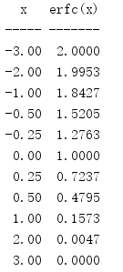
The complementary error function erfc() generates a value equivalent to 1 - erf(x).
import math

print('{:^5} {:7}'.format('x', 'erfc(x)'))
print('{:-^5} {:-^7}'.format('', ''))

for x in [-3, -2, -1, -0.5, -0.25, 0, 0.25, 0.5, 1, 2, 3]:
    print('{:5.2f} {:7.4f}'.format(x, math.erfc(x)))
If the value of x is very small, the implementation of erfc() can avoid the possible precision error when subtracting from 1.