logistic regression
logistic regression
Task 1 Visualization Data (Selection)
The data in ex2data1.txt has been imported into the ex2.m file. The code is as follows:
data = load('ex2data1.txt');
X = data(:, [1, 2]);
y = data(:, 3);
We only need to complete the plotData() function code in the plotData.m file. The code is as follows:
positive = find(y==1);
negative = find(y==0);

plot(X(positive, 1), X(positive, 2), 'k+', 'LineWidth', 2, 'MarkerSize', 7);
plot(X(negative, 1), X(negative, 2), 'ko', 'MarkerFaceColor', 'y','MarkerSize', 7);
Among them, the application of plot() function involved in this code can see my own Octave Course (4) Or consult the relevant documents on your own.
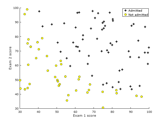
Running part of the task code results in the following figure:
Task two-cost function and gradient descent algorithm
In the ex2.m file, the initialization code of the relevant parameters and the function call code have been written. The code is as follows:
[m, n] = size(X);

% Add intercept term to x and X_test
X = [ones(m, 1) X];

% Initialize fitting parameters
initial_theta = zeros(n + 1, 1);

% Compute and display initial cost and gradient
[cost, grad] = costFunction(initial_theta, X, y);
We only need to complete the cost function and gradient descent algorithm code in costFunction.m. But before that, we need to complete the sigmoid() function in the sigmoid.m file.
First, we will list the formulas to be used:
- Suppose the function h theta(x):

- Cost function J( theta):

Its vectorization is:

- Gradient descent algorithm:
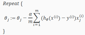
Its vectorization is:

Then, in the sigmoid.m file, we type the following code according to the hypothetical function htheta (x):
g = 1 ./ (1+exp(-z));
Finally, in the costFunction.m file, we complete the cost function J (theta) and the gradient descent algorithm respectively. The codes are as follows:
Cost function J( theta)
J = (-y'*log(sigmoid(X*theta))-(1-y)'*log(1-sigmoid(X*theta))) / m;
Gradient descent algorithm
grad = (X'*(sigmoid(X*theta)-y)) / m;
Running this part of the code results in:
Cost at initial theta (zeros): 0.693147
Expected cost (approx): 0.693
Gradient at initial theta (zeros):
 -0.100000
 -12.009217
 -11.262842
Expected gradients (approx):
 -0.1000
 -12.0092
 -11.2628

Cost at test theta: 0.218330
Expected cost (approx): 0.218
Gradient at test theta:
 0.042903
 2.566234
 2.646797
Expected gradients (approx):
 0.043
 2.566
 2.647
Task Three Advanced Optimization Algorithms
In the ex2.m file, the relevant code using fminunc() function has been written. We just need to run it. The code is as follows:
%  Set options for fminunc
options = optimset('GradObj', 'on', 'MaxIter', 400);

%  Run fminunc to obtain the optimal theta
%  This function will return theta and the cost
[theta, cost] = ...
    fminunc(@(t)(costFunction(t, X, y)), initial_theta, options);

% Print theta to screen
fprintf('Cost at theta found by fminunc: %f\n', cost);
fprintf('Expected cost (approx): 0.203\n');
fprintf('theta: \n');
fprintf(' %f \n', theta);
fprintf('Expected theta (approx):\n');
fprintf(' -25.161\n 0.206\n 0.201\n');

% Plot Boundary
plotDecisionBoundary(theta, X, y);

% Put some labels
hold on;
% Labels and Legend
xlabel('Exam 1 score')
ylabel('Exam 2 score')

% Specified in plot order
legend('Admitted', 'Not admitted')
hold off;
The results of this task are as follows:
Cost at theta found by fminunc: 0.203498
Expected cost (approx): 0.203
theta:
 -25.161272
 0.206233
 0.201470
Expected theta (approx):
 -25.161
 0.206
 0.201

Prediction of Logical Regression in Task Four
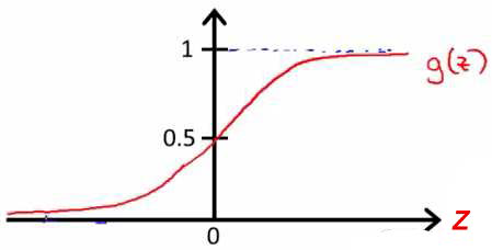
According to the logic function g(z), we can see that:
- When z is greater than or equal to 0.5, we can predict y=1.
- When z is less than 0.5, we can predict y=0.
Therefore, based on the above conclusions, we can complete the predict() function code in the predict.m file, which is as follows:
p(sigmoid( X * theta) >= 0.5) = 1;
p(sigmoid( X * theta) < 0.5) = 0;
Here the code can be broken down into the following code for easy understanding:
k = find(sigmoid( X * theta) >= 0.5 );
p(k)= 1;

d = find(sigmoid( X * theta) < 0.5 );
p(d)= 0;
The results of this task are as follows:
For a student with scores 45 and 85, we predict an admission probability of 0.776289
Expected value: 0.775 +/- 0.002

Train Accuracy: 89.000000
Expected accuracy (approx): 89.0
Logical Regression of Regularization
Task 1 Visualization Data
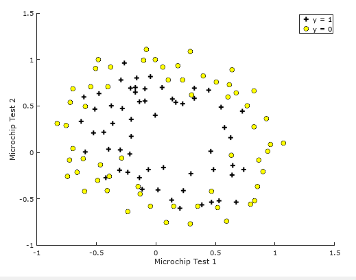
Since the relevant code has been written in ex2_reg.m file and plotData.m file, we only need to run the task code, and the result is as follows:
Task two-cost function and gradient descent algorithm
Regularized cost function J( theta):

Regularized gradient descent algorithm:
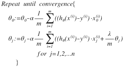
According to the above formula, we can complete the cost function and gradient descent algorithm in costFunctionReg.m file. The code is as follows:
theta_s = [0; theta(2:end)];
J= (-1 * sum( y .* log( sigmoid(X*theta) ) + (1 - y ) .* log( (1 - sigmoid(X*theta)) ) ) / m) + (lambda / (2*m) * (theta_s' * theta_s));
grad = ( X' * (sigmoid(X*theta) - y ) )/ m + ((lambda/m)*theta_s);
Its operation results are as follows:
Cost at initial theta (zeros): 0.693147
Expected cost (approx): 0.693
Gradient at initial theta (zeros) - first five values only:
 0.008475
 0.018788
 0.000078
 0.050345
 0.011501
Expected gradients (approx) - first five values only:
 0.0085
 0.0188
 0.0001
 0.0503
 0.0115

Program paused. Press enter to continue.

Cost at test theta (with lambda = 10): 3.164509
Expected cost (approx): 3.16
Gradient at test theta - first five values only:
 0.346045
 0.161352
 0.194796
 0.226863
 0.092186
Expected gradients (approx) - first five values only:
 0.3460
 0.1614
 0.1948
 0.2269
 0.0922
Task Three Advanced Optimization Algorithms
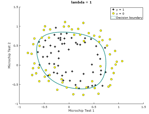
The code has been written and we just need to run it. The result is as follows:
Train Accuracy: 83.050847
Expected accuracy (with lambda = 1): 83.1 (approx)
Task 4: Select regularization parameter lambda (optional)
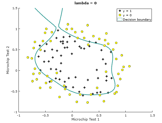
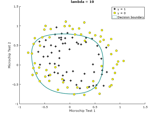
We make the regularization parameters lambda = 0, 10, 100 respectively, and the results are as follows:
λ=0
Train Accuracy: 86.440678
λ=10
Train Accuracy: 74.576271
λ=100
Train Accuracy: 61.016949
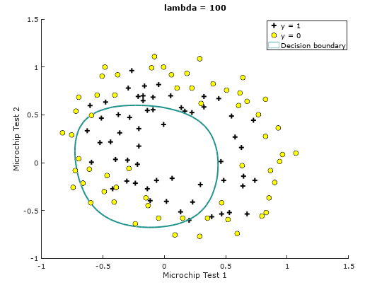
For image rendering, please view the plotDecisionBoundary.m file by yourself.