Source: Data STUDIO

Author: Yun Duojun

1. Brier Score

The accuracy of probability prediction is called "calibration degree", which is a way to measure the difference between the probability predicted by the algorithm and the real result. A commonly used indicator is called Brill score, which is calculated as the mean square error of probability prediction relative to the test sample, expressed as:

Where is the number of samples. It is the probability predicted by the probability model. It is the real result corresponding to the sample. It can only be 0 or 1. If the event occurs, it is 1. If it does not occur, it is 0.

This indicator measures the difference between the probability distance and the real label results. The Brill score ranges from 0 to 1. The higher the score, the worse the prediction result and the worse the calibration degree. Therefore, the closer the Brill score is to 0, the better.

Brier for sklearn_ score_ Loss representation

sklearn.metrics.brier_score_loss(y_true, 
                                 y_prob, 
                                 *, 
                                 sample_weight=None, 
                                 pos_label=None)

• y_ True: array, shape (n_samples,) real label
• y_ Prob: probability value predicted by array, shape (n_samples,)
• sample_ Weight: array like of shape = [n_samples], optional sample weight
• pos_label: int or STR, default = none by default, if label={0,1} or label={-1,1}, the parameter pos_label can be omitted and the default value is used. If label={1,2} is not a standard type, pos_label must be equal to 2. Generally, it is considered that the smaller value is a negative sample label and the larger value is a positive sample label

Brill scores can be used for any prediction that can be used_ The model of probabilities of proba interface calls.

Author: CDA Data Analyst
 Link: https://zhuanlan.zhihu.com/p/391400190
 Source: Zhihu
 The copyright belongs to the author. For commercial reprint, please contact the author for authorization, and for non-commercial reprint, please indicate the source.

import numpy as np
import matplotlib.pyplot as plt
from sklearn.naive_bayes import GaussianNB
from sklearn.datasets import load_digits
from sklearn.model_selection import train_test_split
from sklearn.metrics import brier_score_loss
from sklearn.svm import SVC
from sklearn.linear_model import LogisticRegression as LR

digits = load_digits()
X, y = digits.data, digits.target
Xtrain,Xtest,Ytrain,Ytest = train_test_split(X,y,test_size=0.3,random_state=420)
gnb = GaussianNB().fit(Xtrain,Ytrain)
# Note that the first parameter is the real label and the second parameter is the predicted probability value
# In the case of secondary classification, the interface is predicted_ Proba returns two columns,
# But SVC interface decision_function returns only one column
# Always pay attention to what probability classifier is used to identify the interfaces for finding confidence and the structure of these interfaces
brier_score_loss(Ytest, gnb.predict_proba(Xtest)[:,1], pos_label=1)
>>> 0.032619662406118764

lr = LR(C=1., solver='lbfgs',max_iter=3000,multi_class="auto").fit(Xtrain,Ytrain)
svc = SVC(kernel = "linear",gamma=1).fit(Xtrain,Ytrain)
brier_score_loss(Ytest,lr.predict_proba(Xtest)[:,1],pos_label=1)
>>> 0.011386864786268255

#Since the confidence of SVC is not probability, for comparability,
# The confidence "distance" of SVC needs to be normalized and compressed to between [0,1]
svc_prob = (svc.decision_function(Xtest) -
svc.decision_function(Xtest).min())/(svc.decision_function(Xtest).max() -
svc.decision_function(Xtest).min())
brier_score_loss(Ytest,svc_prob[:,1],pos_label=1)
>>> 0.23818950248917947

Visualize Brill scores under each label category for each classifier:

Author: CDA Data Analyst
 Link: https://zhuanlan.zhihu.com/p/391400190
 Source: Zhihu
 The copyright belongs to the author. For commercial reprint, please contact the author for authorization, and for non-commercial reprint, please indicate the source.

import pandas as pd
name = ["Bayes","Logistic","SVC"]
color = ["red","black","orange"]
df = pd.DataFrame(index=range(10),columns=name)
for i in range(10):
    df.loc[i,name[0]] = brier_score_loss(Ytest,gnb.predict_proba(Xtest)[:,i],pos_label=i)
    df.loc[i,name[1]] = brier_score_loss(Ytest,lr.predict_proba(Xtest)[:,i],pos_label=i)
    df.loc[i,name[2]] = brier_score_loss(Ytest,svc_prob[:,i],pos_label=i)
plt.figure(figsize=(16,6))
for i in range(df.shape[1]):
    plt.plot(range(10),df.iloc[:,i],c=color[i],label=name[i])
plt.legend(fontsize=20,loc='upper left')
plt.show()

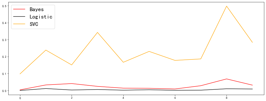
It can be observed that the Brill score of logistic regression has an overwhelming advantage, and the effect of SVC is significantly weaker than that of Bayesian and logistic regression (SVC forcibly uses sigmoid function to compress the probability, so the probability result produced by SVC is not so reliable). Bayesian is between logistic regression and SVC, and the effect is also good, but it is not accurate and stable compared with logistic regression.

2. Log Loss of log likelihood function

For a given probability classifier, the negative logarithm of the probability of the occurrence of the real probability under the condition of the prediction probability. Here you can refer to logistic regression.

Because it is a loss, the smaller the value of log likelihood function is, the more accurate the probability estimation is and the more ideal the model is. Logarithmic loss can only be used to evaluate sub type models.

For a sample, if the true label of the sample is taken in {0,1} and the probability of the sample under Category 1 is estimated as, the corresponding logarithmic loss of the sample is:

sklearn.metrics.log_loss(y_true, 
                         y_pred, 
                         *, 
                         eps=1e-15,
                         normalize=True, 
                         sample_weight=None, 
                         labels=None)

• y_ True: array like or label indicator is the real label of the matrix sample
• y_ PRED: array like of float, shape = (n_samples, n_classes) or (n_samples,) prediction probability. Be careful not to mistake the prediction label for the interface predict_proba to call
• EPS: float precision
• Normalize: bool, optional (default = true). If true, the average loss of each sample is returned. Otherwise, return the sum of the losses for each sample.
• sample_ Weight: array like of shape (n_samples,), default = none
• Labels: array like, optional (default = None) if it is not provided, it will start from y_true infers the label. If the label is None and y_pred has shapes (n_samples), it is assumed that the label is binary and from y_true infers.

>>> from sklearn.metrics import log_loss
# Gaussian Bayes
>>> log_loss(Ytest,gnb.predict_proba(Xtest))
2.4725653911460683
# logistic regression 
>>> log_loss(Ytest,lr.predict_proba(Xtest))
0.12738186898609435
# Support vector machine
>>> log_loss(Ytest,svc_prob)
1.625556312147472

Use log_ The conclusion drawn by loss is inconsistent with the conclusion drawn by Brill score: when Brill score is used as the evaluation standard, the estimation effect of SVC is the worst, and the results of logistic regression and Bayesian are close. When using log likelihood, although logistic regression is still the most powerful, Bayesian is not as effective as SVC. Why is there such a difference?

Because both logistic regression and SVC are algorithms to solve the model for the purpose of optimization and then classify. In naive Bayes, however, there is no optimization process. Log likelihood function directly points to the direction of model optimization, even the loss function of logistic regression itself, so it performs better in logistic regression and SVC.

When to use log likelihood and Brill fraction?

In practical applications, log likelihood function is the golden index for the evaluation of probability models and the preferred choice for the evaluation of probability models. But it also has some disadvantages.

• Firstly, it has no boundary, unlike Brill's score, which has an upper limit, and can be used as a reference for the effect of the model.
• Secondly, its interpretability is not as good as Brill score, so it is difficult to communicate the reliability and necessity of log likelihood with non-technical personnel.
• Third, it performs better in the model aiming at optimization. Moreover, it also has some mathematical problems, such as the probability of 0 or 1 cannot be accepted, otherwise the log likelihood will reach the limit value

3. Reliability Curve

The algorithm of output probability has its own adjustment method, which is to adjust the calibration degree of probability. The higher the degree of calibration, the more accurate the probability prediction of the model, the more confident the algorithm is in making judgment, and the more stable the model will be.

reliability curve, also known as probability calibration curve and reliability diagrams, is a curve with predicted probability as abscissa and real label as ordinate.

It is hoped that the closer the predicted probability is to the real value, the better. It is better that they are equal. Therefore, the closer the probability calibration curve of a model / algorithm is to the diagonal, the better. The calibration curve is therefore one of the model evaluation indicators. Similar to Brill score, the probability calibration curve is for a certain class of labels, so a class of labels will have a curve, or we can use the average under a multi class label to represent the probability calibration curve of the whole model.

sklearn.calibration.calibration_curve(y_true, 
                                      y_prob, 
                                      *, 
                                      normalize=False, 
                                      n_bins=5, 
                                      strategy='uniform')

• y_ True: array, shape (n_samples,) real label
• y_ Prob: array, shape (n_samples,) predicts the returned probability value or confidence under the positive category
• Normalize: bool, optional, default = False, Boolean, default = False. Do you want to y_ The input content in prob is normalized to [0, 1], when y_prob can be used when it is not a real probability. If the parameter is True, y is set_ The minimum value in prob is normalized to 0 and the maximum value is normalized to 1.
• n_ Bins: int integer value, indicating the number of bins. If the number of boxes is large, more data is required.

return

• The ordinate of trueproba reliability curve, with the structure of (n_bins,), is the proportion of a few classes (Y=1) in each box
• The abscissa of the predproba reliability curve, with the structure of (n_bins,), is the mean value of the probability in each box

Reliability curve drawing

import numpy as np
import matplotlib.pyplot as plt
from sklearn.datasets import make_classification as mc
from sklearn.naive_bayes import GaussianNB
from sklearn.svm import SVC
from sklearn.linear_model import LogisticRegression as LR
from sklearn.metrics import brier_score_loss
from sklearn.model_selection import train_test_split
from sklearn.calibration import calibration_curve

X, y = mc(n_samples=100000,n_features=20 #Total 20 features
          ,n_classes=2 #The label is classified as 2
          ,n_informative=2 #Two of them represent more information
          ,n_redundant=10 #All 10 are redundant features
          ,random_state=42)
#The sample size is large enough, so 1% of the samples are used as the training set
Xtrain, Xtest, Ytrain, Ytest = train_test_split(X, y, test_size=0.99, random_state=42)

Model establishment and reliability curve drawing

Author: CDA Data Analyst
 Link: https://zhuanlan.zhihu.com/p/391400190
 Source: Zhihu
 The copyright belongs to the author. For commercial reprint, please contact the author for authorization, and for non-commercial reprint, please indicate the source.

gnb = GaussianNB()
gnb.fit(Xtrain,Ytrain)
gnb_score = gnb.score(Xtest, Ytest)
y_pred = gnb.predict(Xtest)
prob = gnb.predict_proba(Xtest)[:,1] #Our prediction probability - abscissa
#Ytest - our real label - abscissa

#From class calibiration_ Obtain abscissa and ordinate from curve
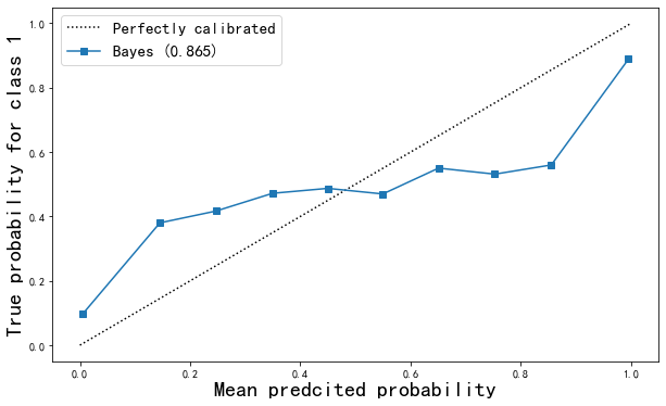
trueproba, predproba = calibration_curve(Ytest, prob ,
                                         n_bins=10 #Enter the number of boxes you want to divide
                                        )
fig = plt.figure(figsize=(10,6))
ax1 = plt.subplot()
ax1.plot([0, 1], [0, 1], "k:", label="Perfectly calibrated")
ax1.plot(predproba, trueproba,"s-",label="%s (%1.3f)" % ("Bayes",gnb_score))
ax1.set_ylabel("True probability for class 1", fontsize=20)
ax1.set_xlabel("Mean predcited probability", fontsize=20)
ax1.set_ylim([-0.05, 1.05])
ax1.legend(fontsize=15)
plt.show()

Different N_ Curve under bins value

fig, axes = plt.subplots(1,3,figsize=(18,5))
for ind,i in enumerate([3,10,100]):
ax = axes[ind]
	ax.plot([0, 1], [0, 1], "k:", label="Perfectly calibrated")
	trueproba, predproba = calibration_curve(Ytest,prob,n_bins=i)
	ax.plot(predproba, trueproba,"s-",label="n_bins = {}".format(i))
	ax1.set_ylabel("True probability for class 1")
	ax1.set_xlabel("Mean predcited probability")
	ax1.set_ylim([-0.05, 1.05])
	ax.legend()plt.show()

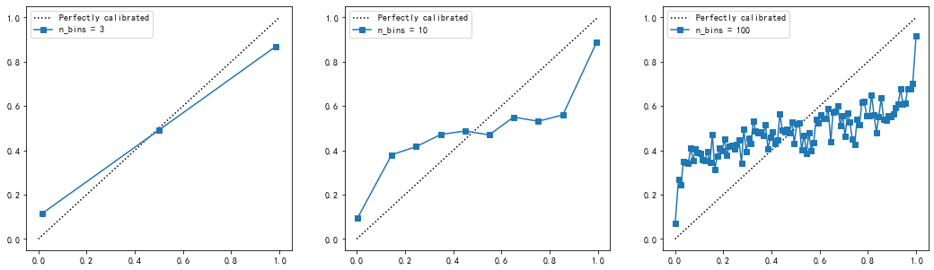
Obviously,

n_ The larger the bins and the more boxes, the more accurate the probability calibration curve will be, but the curve that is too accurate is not smooth enough to be compared with the perfect probability density curve we want.

n_ The smaller the bins and the fewer boxes, the coarser the probability calibration curve. Although it is close to the perfect probability density curve, it can not truly show the results of model probability prediction.

Therefore, we need to take a number of boxes that are neither too large nor too small, so that the probability calibration curve is neither too accurate nor too rough, but a relatively smooth curve that can reflect the trend of the model's probability prediction. Generally speaking, it is recommended to try the case where the number of boxes is equal to 10. The larger the number of boxes, the more sample size is required, otherwise the curve will be too accurate.

Comparison of different models

X, y = mc(n_samples=100000,n_features=20 #Total 20 features
          ,n_classes=2 #The label is classified as 2
          ,n_informative=2 #Two of them represent more information
          ,n_redundant=10 #All 10 are redundant features
          ,random_state=42)
#The sample size is large enough, so 1% of the samples are used as the training set
Xtrain, Xtest, Ytrain, Ytest = train_test_split(X, y,test_size=0.99,random_state=42)
gnb = GaussianNB()
lr = LR(C=1., solver='lbfgs',max_iter=3000,multi_class="auto")
svc = SVC(kernel = "linear",gamma=1)
names = ["GaussianBayes","Logistic","SVC"]
clfs=[gnb,lr,svc]
fig, ax1 = plt.subplots(figsize=(10,5))
ax1.plot([0, 1], [0, 1], "k:", label="Perfectly calibrated")
for clf, name in zip(clfs,names):
    print(name)
    clf.fit(Xtrain,Ytrain)
    y_pred = clf.predict(Xtest)
    #hasattr(obj,name): check whether an interface named name exists in a class obj. If it exists, it returns True
    if hasattr(clf, "predict_proba"):
        prob = clf.predict_proba(Xtest)[:,1]
    else: # use decision function
        prob= clf.decision_function(Xtest)
        prob= (prob - prob.min()) / (prob.max() - prob.min())
    #Return Brill score
    clf_score = brier_score_loss(Ytest, prob, pos_label=y.max())
    trueproba, predproba = calibration_curve(Ytest, prob,n_bins=10)
    ax1.plot(predproba, trueproba,"s-",label="%s (%1.3f)" % (name, clf_score))
    
ax1.set_ylabel("True probability for class 1")
ax1.set_xlabel("Mean predcited probability")
ax1.set_ylim([-0.05, 1.05])
ax1.legend()
ax1.set_title('Calibration plots (reliability curve)')
plt.show()

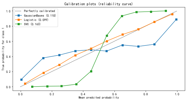
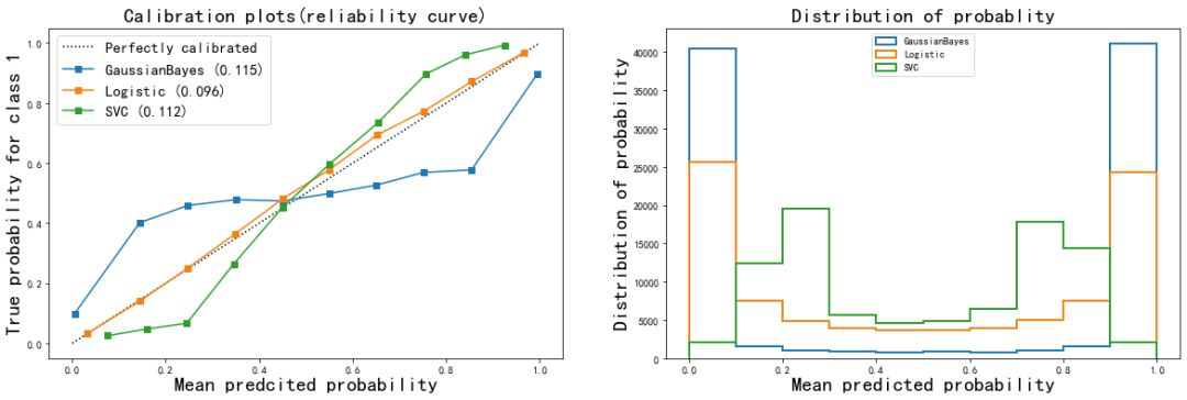
It can be seen from the results of the image

• The probability estimation of logistic regression is the closest to the perfect probability calibration curve, so the effect of logistic regression is the most perfect.
• The results of Gaussian naive Bayes and support vector machine classifiers are poor.
• Support vector machine presents a shape similar to sigmoid function. The effect of its probability calibration curve is the performance of a typical under confidence classifier: a large number of sample points are concentrated near the decision boundary, and their confidence is close to about 0.5. Even if the decision boundary can judge the sample points correctly, the model itself is not very sure of this result. In contrast, the confidence of the point far from the decision boundary will be very high, because it is very likely that it will not be misjudged. Support vector machine (SVM) has the inherent disadvantage of insufficient confidence when facing mixed data.
• Gaussian naive Bayes presents the opposite shape of Sigmoid function, indicating that the features in the data set are not conditionally independent of each other. This is related to the data set we set, in which the 10 redundant features are not completely independent.

4. Histogram of prediction probability

You can draw a histogram to view the distribution of the prediction probability of the model. Histogram is an image with the predicted probability of samples as the abscissa and the number of samples in each box as the ordinate.

fig, ax2 = plt.subplots(figsize=(10,6))
for clf, name in zip(clfs,names):
    clf.fit(Xtrain,Ytrain)
    y_pred = clf.predict(Xtest)
    if hasattr(clf, "predict_proba"):
        prob = clf.predict_proba(Xtest)[:,1]
    else: # use decision function
        prob = clf.decision_function(Xtest)
        prob = (prob - prob.min()) / (prob.max() - prob.min())
    ax2.hist(prob
             ,bins=10
             ,label=name
             ,histtype="step" #Set histogram to transparent
             ,lw=2 #Set the stroke thickness of each column in the histogram
             )
ax2.set_ylabel("Distribution of probability", fontsize=20)
ax2.set_xlabel("Mean predicted probability", fontsize=20)
ax2.set_xlim([-0.05, 1.05])
ax2.set_xticks([0,0.1,0.2,0.3,0.4,0.5,0.6,0.7,0.8,0.9,1])
ax2.legend(loc=9, fontsize=15)
plt.show()

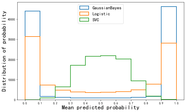
Can see

• The probability distribution of Gaussian Bayesian is very high on both sides and very low in the middle. Almost more than the samples are near 0 and 1, which can be said to be the algorithm with the highest confidence. However, the Brill score of Bayesian is not as good as logistic regression, which proves that some samples near 0 and 1 in Bayesian are misclassified.
• Support vector Bayes is completely opposite, which is obviously high in the middle and low on both sides, which is similar to the normal distribution. It is proved that most samples are near the decision boundary and the confidence hovers around 0.5 as shown in the reliability curve.
• Logistic regression is located between Gaussian naive Bayes and support vector machine, that is, not too many samples are too close to 0 and 1, nor does it form a normal distribution like support vector machine. The probability distribution of a relatively healthy positive sample.

5. Calibration reliability curve

There are two kinds of isoparametric regression, one is the parameter calibration method of Sigmoid model based on Platt, and the other is the nonparametric calibration method based on isotonic calibration. Probabilistic calibration should occur on the test set and must be data that the model has never seen.

Mathematically, the principle of using these two methods to calibrate probability is very complex, and we can't interfere in this process in sklearn, so we don't have to study it too deeply.

class sklearn.calibration.CalibratedClassifierCV (base_estimator=None,
                                                  method='sigmoid',
                                                  cv='warn')

This is a probability calibration class with cross validation. It uses the cross validation generator to estimate the model parameters on the training samples for each data in the cross validation, conduct probability calibration on the test samples, and then return the best set of parameter estimation and calibration results for us. The prediction probability of each data is averaged. Note that the class CalibratedClassifierCV has no interface decision_function, to view the generation probability of the calibrated model under this class, you must call predict_proba interface.

• base_estimator=None: the classifier whose output decision function needs to be calibrated must have a "predict_proba" or "decision_function" interface. If the parameter "CV = prefix", the classifier must have fitted the data.
• Method = "sigmoid": the method for probability calibration. You can enter "sigmoid" or "isotonic". Input 'sigmoid', use the sigmoid model based on Platt for calibration, and input 'isotonic', use isotonic regression for calibration. When the calibration sample size is too small (for example, less than or equal to 1000 test samples), isotonic regression is not recommended because it tends to over fitting. When the sample size is too small, please use sigmoids, i.e. Platt calibration.
• CV = 'warn' integer, which determines the cross validation strategy. The possible input is: None, which means the default 50% off cross validation is used. Any integer, specifying the discount. For the input integer and None, if it is binary classification, the class sklearn.model is automatically used_ Selection.stratifiedkfold performs fold segmentation. If y is a continuous variable, use sklearn.model_selection.KFold for segmentation. Cross validation patterns or generators built using other classes cv. Iterative, segmented test set and training set index array. If you enter "prefix", it is assumed that the data has been fitted on the classifier. In this mode, the user must manually determine that the data used to fit the classifier does not intersect with the data to be calibrated.

# Encapsulating visualization functions
def plot_calib(models,names,Xtrain,Xtest,Ytrain,Ytest,n_bins=10):
    import matplotlib.pyplot as plt
    from sklearn.metrics import brier_score_loss
    from sklearn.calibration import calibration_curve
    fig, (ax1, ax2) = plt.subplots(1, 2,figsize=(20,6))
    ax1.plot([0, 1], [0, 1], "k:", label="Perfectly calibrated")
    for clf, name in zip(models,names):
        clf.fit(Xtrain,Ytrain)
        y_pred = clf.predict(Xtest)
    #hasattr(obj,name): check whether an interface named name exists in a class obj. If it exists, it returns True
        if hasattr(clf, "predict_proba"):
            prob = clf.predict_proba(Xtest)[:,1]
        else: # use decision function
            prob = clf.decision_function(Xtest)
            prob = (prob - prob.min()) / (prob.max() - prob.min())
        #Return Brill score
        clf_score = brier_score_loss(Ytest, prob, pos_label=y.max())
        trueproba, predproba = calibration_curve(Ytest, prob,n_bins=n_bins)
        ax1.plot(predproba, trueproba,"s-",label="%s (%1.3f)" % (name, clf_score))
        ax2.hist(prob, range=(0, 1), bins=n_bins, label=name, histtype="step", lw=2)
    ax2.set_ylabel("Distribution of probability", fontsize=20)
    ax2.set_xlabel("Mean predicted probability", fontsize=20)
    ax2.set_xlim([-0.05, 1.05])
    ax2.legend(loc=9)
    ax2.set_title("Distribution of probablity", fontsize=20)
    ax1.set_ylabel("True probability for class 1", fontsize=20)
    ax1.set_xlabel("Mean predcited probability", fontsize=20)
    ax1.set_ylim([-0.05, 1.05])
    ax1.legend(fontsize=15)
    ax1.set_title('Calibration plots(reliability curve)', fontsize=20)
    plt.show()

# Model preparation
from sklearn.calibration import CalibratedClassifierCV
names = ["GaussianBayes","Logistic","SVC"]
models = [GaussianNB()
          ,LR(C=1., solver='lbfgs',max_iter=3000,multi_class="auto")
          #Define two calibration methods
          ,SVC(kernel = 'rbf')]
# Data preparation
X, y = mc(n_samples=100000,n_features=20 #Total 20 features
         ,n_classes=2 #The label is classified as 2
         ,n_informative=2 #Two of them represent more information
         ,n_redundant=10 #All 10 are redundant features
         ,random_state=42)

Xtrain,Xtest,Ytrain,Ytest = train_test_split(X,y,test_size = 0.9,random_state = 0)

# Function execution
plot_calib(models,names,Xtrain,Xtest,Ytrain,Ytest)

View changes in accuracy based on calibration results

gnb = GaussianNB().fit(Xtrain,Ytrain)
gnb.score(Xtest,Ytest)
>>> 0.8669222222222223
brier_score_loss(Ytest,gnb.predict_proba(Xtest)[:,1],pos_label = 1)
>>> 0.11514876553209971
gnbisotonic = CalibratedClassifierCV(gnb, cv=2, method='isotonic').fit(Xtrain,Ytrain)
gnbisotonic.score(Xtest,Ytest)
>>> 0.8665111111111111
brier_score_loss(Ytest,gnbisotonic.predict_proba(Xtest)[:,1],pos_label = 1)
>>> 0.09576140551554904

It can be seen that after the calibration probability, the Brill score decreases obviously, but the overall accuracy decreases slightly, which proves that after the calibration, although the prediction of the probability is more accurate, the judgment of the model decreases slightly.

Comparison of calibration results of different models

GaussianNB_CCC = [GaussianNB()
                  ,CalibratedClassifierCV(GaussianNB(),method = 'sigmoid',cv=5)
                  ,CalibratedClassifierCV(GaussianNB(),method = 'isotonic',cv=5)
                  ]
LR_CCC = [LR(solver = 'lbfgs',max_iter = 3000,multi_class = 'auto')
          ,CalibratedClassifierCV(LR(solver = 'lbfgs',max_iter = 3000,multi_class = 'auto'),method = 'sigmoid',cv=5)
          ,CalibratedClassifierCV(LR(solver = 'lbfgs',max_iter = 3000,multi_class = 'auto'),method = 'isotonic',cv=5)
          ]
SVC_CCC = [SVC(kernel = 'rbf',gamma='scale')
           ,CalibratedClassifierCV(SVC(kernel = 'rbf',gamma='scale'),method = 'sigmoid',cv = 5)
           ,CalibratedClassifierCV(SVC(kernel = 'rbf',gamma='scale'),method = 'isotonic',cv = 5)
           ]
estimators_CCC = [GaussianNB_CCC,LR_CCC,SVC_CCC]

GaussianNB_names =['GaussianNB','GaussianNB+sigmoid','GaussianNB+isotonic']
LR_names = ['LogisticRegression','LogisticRegression+sigmoid','LogisticRegression+isotonic']
SVC_names = ['SVC','SVC+sigmoid','SVC+isotonic']
names = [GaussianNB_names,LR_names,SVC_names]

for i in range(len(estimators_CCC)):
    plot_calib(estimators_CCC[i],names[i],Xtrain,Xtest,Ytrain,Ytest)

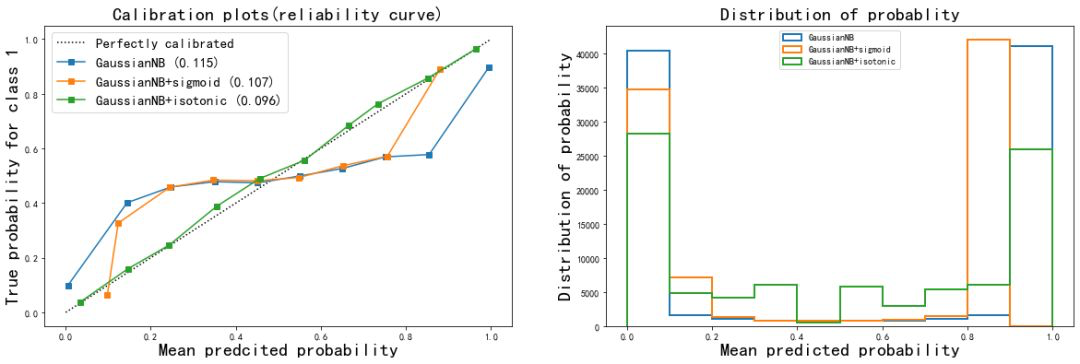
From the correction results:

• The Isotonic isoosmotic correction of naive Bayes greatly improved the shape of the curve, almost made the effect of Bayes equal to that of logistic regression, and the Brill score also decreased to 0.096. Sigmoid calibration method also slightly improves the curve, but the effect is not obvious. From the histogram, Isotonic correction makes the effect of Gaussian naive Bayes close to logistic regression, while the result after sigmoid correction is still closer to the original Gaussian naive Bayes.
• It can be seen that when the features of the data are not conditionally independent of each other, using Isotonic method to calibrate the probability curve can get good results and make the model more modest in prediction
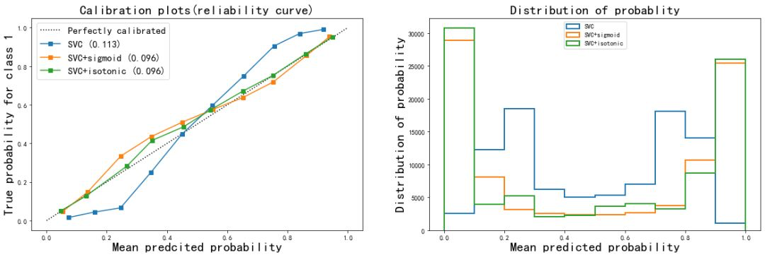
• For SVC, both corrections improve the accuracy and Brill score. It can be seen that probability correction is very effective for SVC. This also shows that the probability correction algorithm is more effective for the original reliability curve to describe the Sigmoid shape curve.
  In reality, you can adjust the model according to your own needs.
• For probabilistic models, there are few adjustable parameters, so we prefer to pursue probabilistic fitting and use probabilistic calibration to adjust the model.
• If you really want to pursue higher accuracy and Recall, you can consider using the naturally very accurate probability class model logistic regression, or you can also consider using the support vector machine classifier with many adjustable parameters in addition to probability calibration.