preface

Bayesian classifier is a probability model, which uses Bayesian formula to solve the classification problem. Assuming that the feature vector of the sample obeys a certain probability distribution, we can calculate the conditional probability that the feature vector belongs to each class. The classification result is the one with the largest conditional probability. If each component of the feature vector is assumed to be independent of each other, it is a naive Bayesian classifier. If the eigenvector is assumed to obey multidimensional normal distribution, it is positive Bayesian.

1. Bayesian decision making

Conditional probability describes the probability relationship between two causal random variables. p(b|a) is defined as the probability of event B under the premise of time a. The Bayesian formula clarifies the probability relationship between two random events:
This conclusion can be extended to random variables. In the classification problem, the value x of the eigenvector has a causal relationship with the category y to which the sample belongs. Because the sample belongs to y, there is characteristic X. For example, in general, an apple is red. Because it is an apple, it has the characteristics of red. On the contrary, our classifier needs to deduce the category of the sample when the feature vector x is known. For example, if the feature of red fruit is known, it is the category of apple. According to Bayesian formula:
As long as we know the probability distribution p(x) of the eigenvector, the probability p(y) of the occurrence of each class, and the conditional probability p(x|y) of the occurrence of each class of samples. The probability p(y|x) that the sample belongs to each class can be calculated. Then find the largest category. The calculation of p(x) is the same for each class, so it can be ignored. The final discriminant function is:
To realize Bayesian classifier, we need to know the probability distribution that the feature vector of each type of sample obeys. In reality, many random variables obey normal distribution, so normal distribution is often used to represent the probability distribution of feature vector. Then we use the maximum likelihood estimation to calculate the two parameters of mean and variance in the normal distribution of each type of sample, and we can get the classification result by calculating the final result of our above discriminant function.

2. About the implementation of sklearn

2.1 Gaussian naive Bayes

Gaussian NB implements the Gaussian naive Bayesian algorithm for classification. The probability (i.e. probability) of the feature is assumed to be Gaussian distribution:

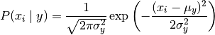
The mean and variance of parameters were estimated by maximum likelihood method.

2.2 naive Bayes of multinomial distribution

MultinomialNB implements a naive Bayesian algorithm for multinomial distributed data, and the parameters are also calculated by maximum likelihood estimation.

2.3 Bernoulli naive Bayes

BernoulliNB implements a naive Bayesian training and classification algorithm for multiple Bernoulli distribution data, that is, there are multiple features, but each feature is assumed to be a binary (Bernoulli, boolean) variable. Therefore, such algorithms require samples to be represented by binary eigenvectors; If the sample contains other types of data, a BernoulliNB instance will binarize it (depending on the binarize parameter).

Bernoulli naive Bayes based decision rules

Different from the rules of multinomial distribution naive Bayes, Bernoulli naive Bayes explicitly penalizes that the feature i as a predictor does not appear in Class y, while multinomial distribution naive Bayes simply ignores the features that do not appear.

Example

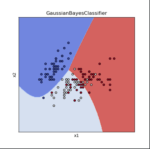
The following is a code using normal naive Bayes classification using iris data set:

import numpy as np
import matplotlib.pyplot as plt
from sklearn import datasets
from sklearn.naive_bayes import GaussianNB
import matplotlib

# Generate all test sample points
def make_meshgrid(x, y, h=.02):
    x_min, x_max = x.min() - 1, x.max() + 1
    y_min, y_max = y.min() - 1, y.max() + 1
    xx, yy = np.meshgrid(np.arange(x_min, x_max, h),np.arange(y_min, y_max, h))
    return xx, yy

# Predict the test sample and display it
def plot_test_results(ax, clf, xx, yy, **params):
    Z = clf.predict(np.c_[xx.ravel(), yy.ravel()])
    Z = Z.reshape(xx.shape)
    #Draw contour lines
    ax.contourf(xx, yy, Z, **params)

# Load iris dataset
iris = datasets.load_iris()
# Use only the first two features
X = iris.data[:, :2]
# Sample tag value
y = iris.target

# Create and train normal naive Bayesian classifier
clf = GaussianNB()
clf.fit(X,y)

title = ('GaussianBayesClassifier')

fig, ax = plt.subplots(figsize = (5, 5))
plt.subplots_adjust(wspace=0.4, hspace=0.4)

#Take out two features respectively
X0, X1 = X[:, 0], X[:, 1]
# Generate all test sample points
xx, yy = make_meshgrid(X0, X1)

# Displays the classification results of the test samples
plot_test_results(ax, clf, xx, yy, cmap=plt.cm.coolwarm, alpha=0.8)
# Show training samples
ax.scatter(X0, X1, c=y, cmap=plt.cm.coolwarm, s=20, edgecolors='k')
ax.set_xlim(xx.min(), xx.max())
ax.set_ylim(yy.min(), yy.max())
ax.set_xlabel('x1')
ax.set_ylabel('x2')
ax.set_xticks(())
ax.set_yticks(())
ax.set_title(title)
plt.show()

The results are as follows: