1, Theoretical learning
Learn the reference material "prediction of house prices by multiple linear regression model. ipynb", and re do the multiple linear regression (based on the statistical analysis library statsmodes) for the house data set "house_prices.csv"; It also focuses on understanding biased data, preprocessing of missing data (data cleaning), detection method of "characteristic collinearity" and traditional estimation parameters of statistics
(1) Background
The Boston house price data set includes multiple samples, and each sample includes multiple characteristic variables and the average house price in the region. House price (unit price) is obviously related to multiple characteristic variables, which is not a univariate linear regression (univariate linear regression) problem; Selecting multiple characteristic variables to establish a linear equation is the problem of multivariable linear regression (multiple linear regression).
House price is related to multiple characteristic variables. This case tries to use multiple linear regression modeling
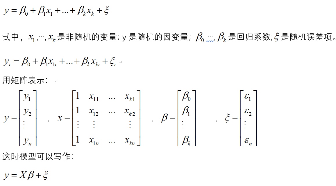
(2) Linear regression test
Under the assumption of normality, if X is full rank, the least squares estimation of the parameters of the ordinary linear regression model is: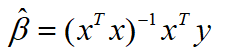
Thus, the estimated value of y is: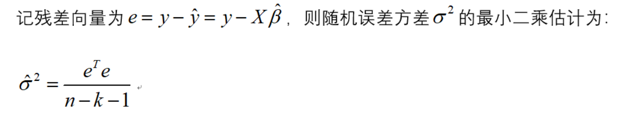
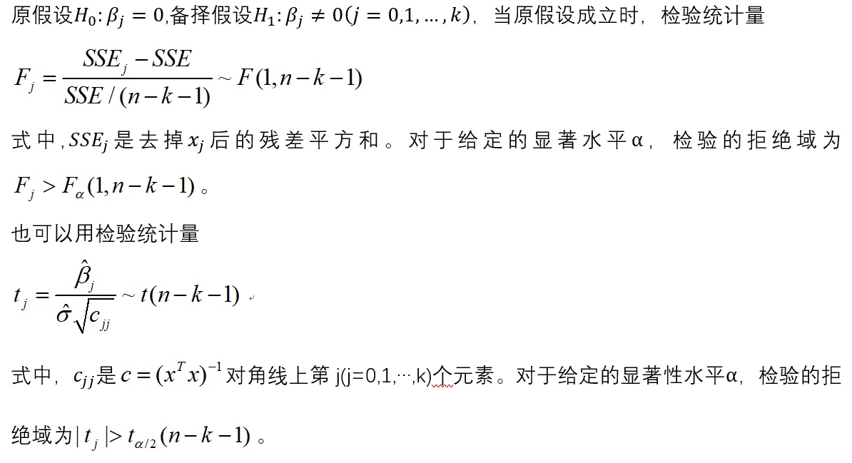
(1) Significance test of regression equation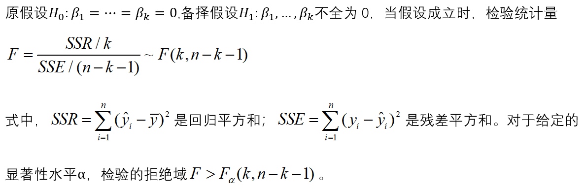
(2) Significance test of regression coefficient
2, Data cleaning
(1) Numerical data processing
1. Main problems of data set
(1) Missing data
(2) Inconsistent data
(3) There is "dirty" data
(4) Nonstandard data
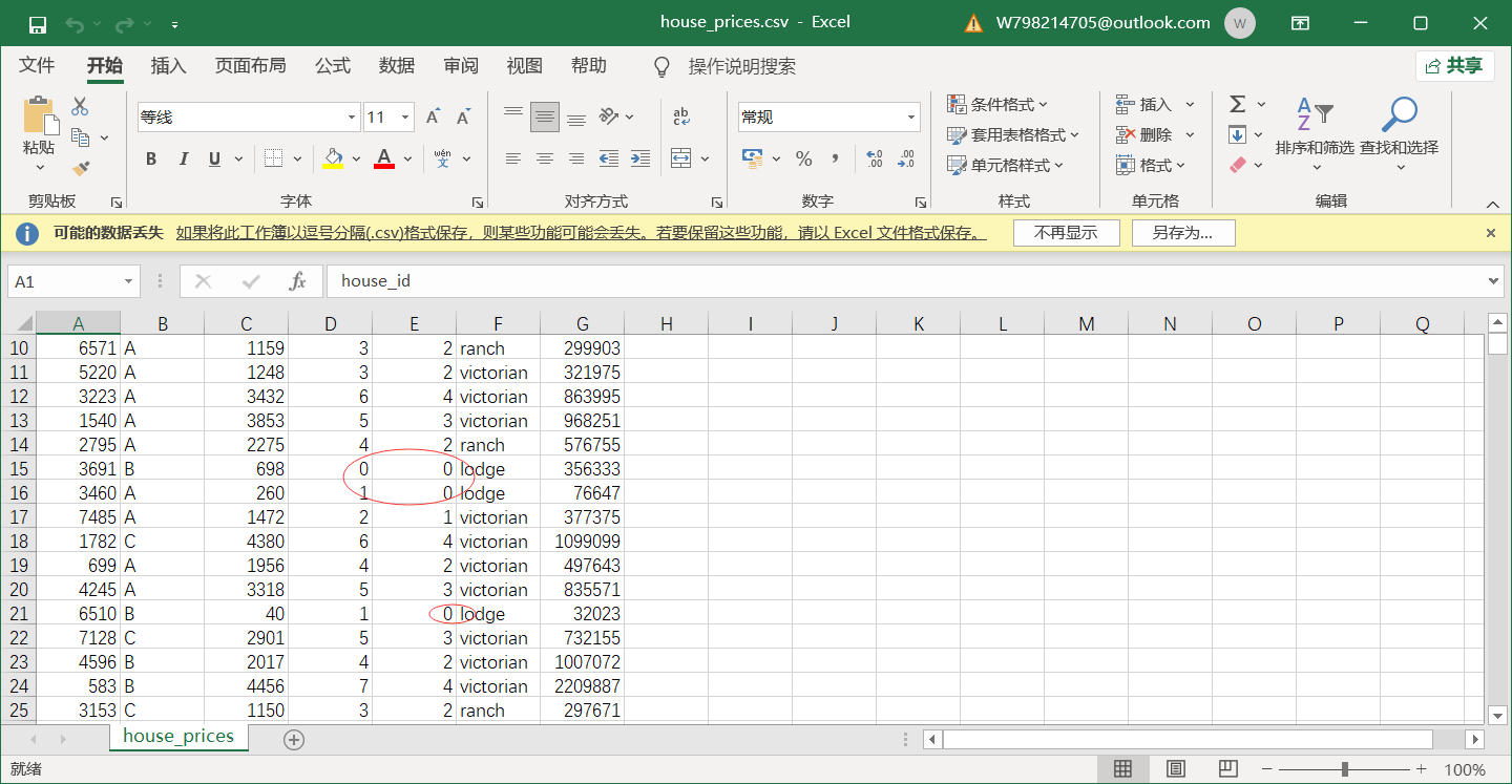
The data is relatively regular as a whole, but through preliminary observation, the data set is mainly missing, and some data are equal to 0.
2. Delete duplicate data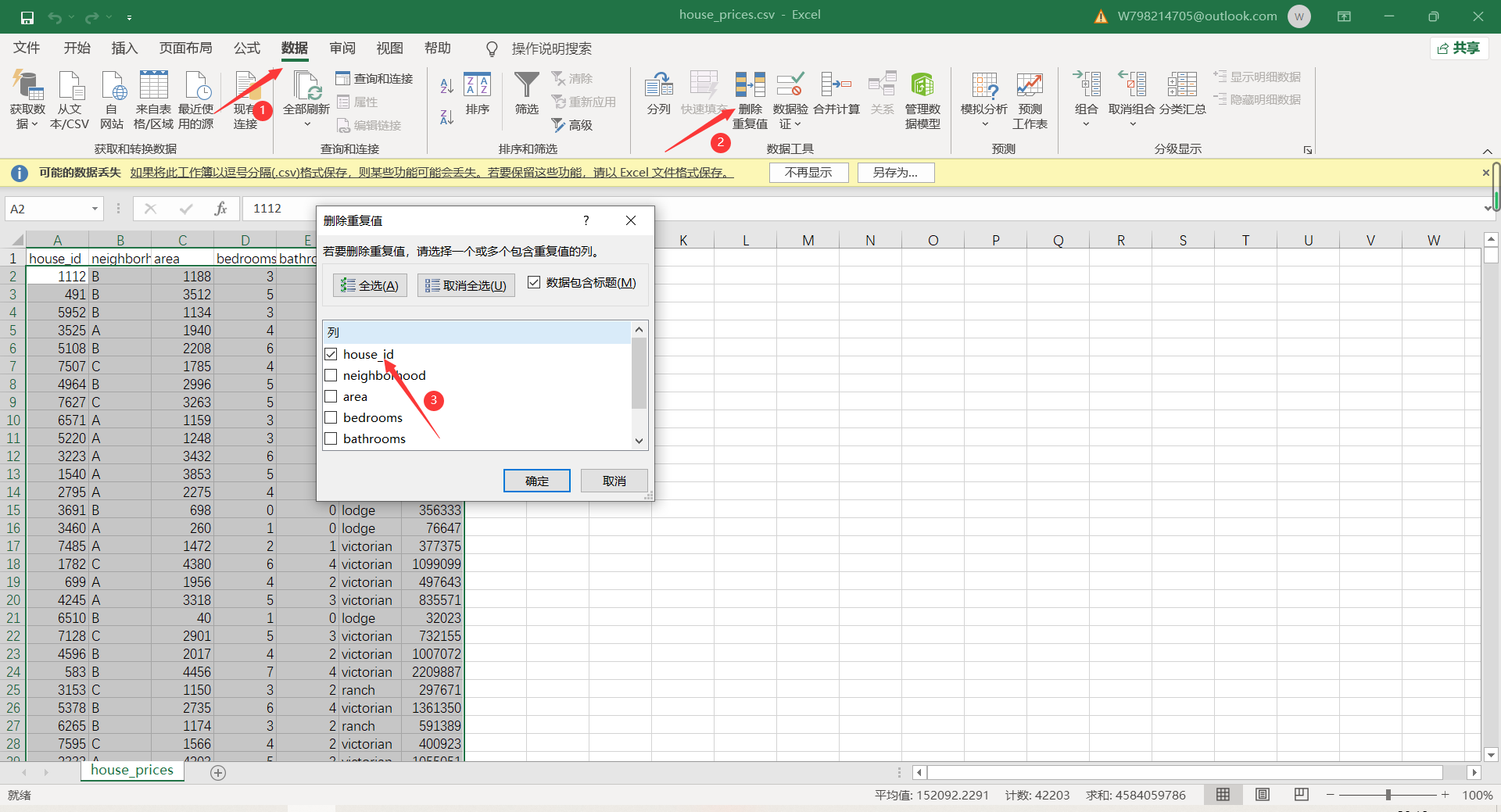
3. Sort in ascending order, select filter and sort - ascending order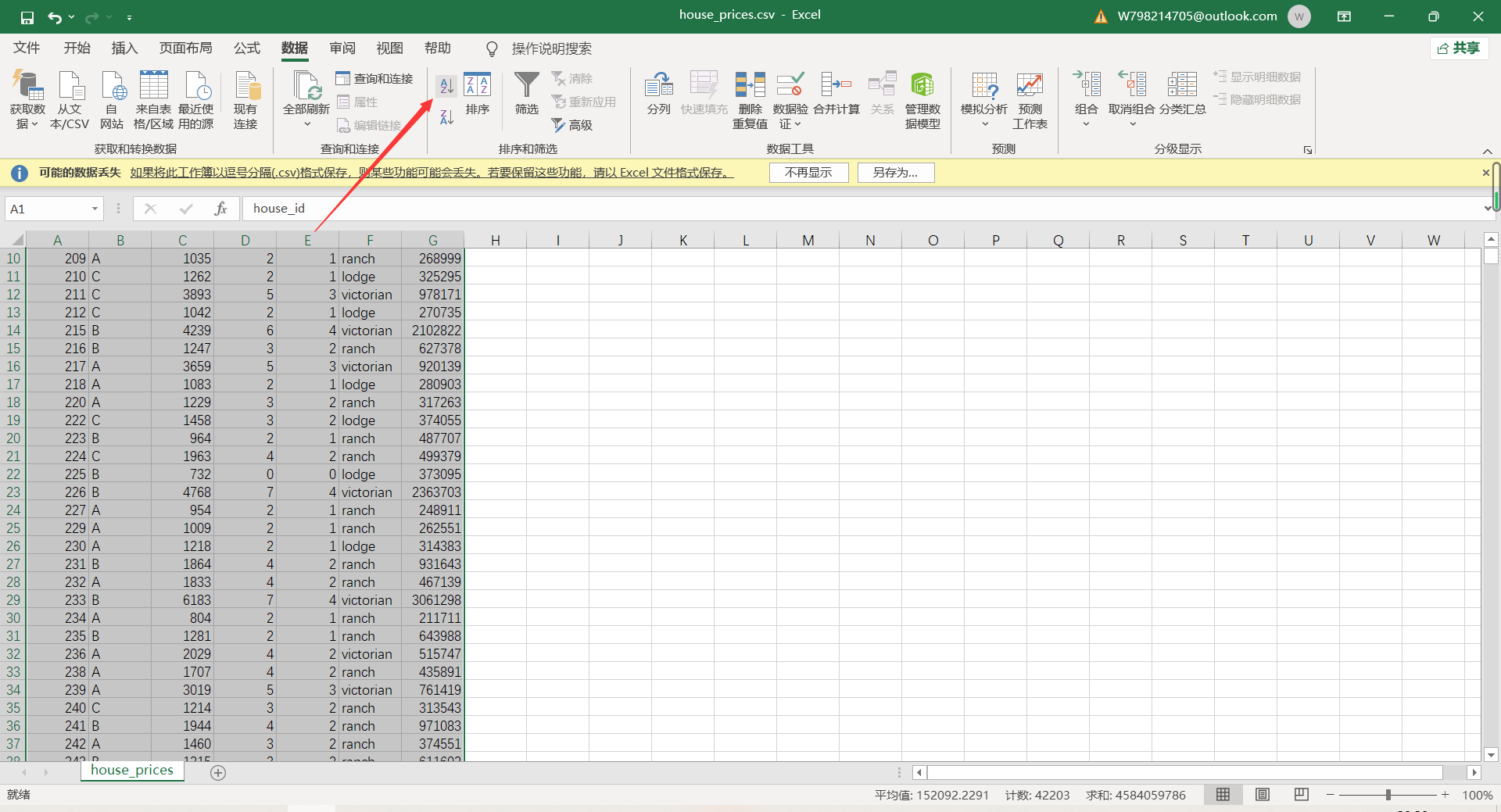
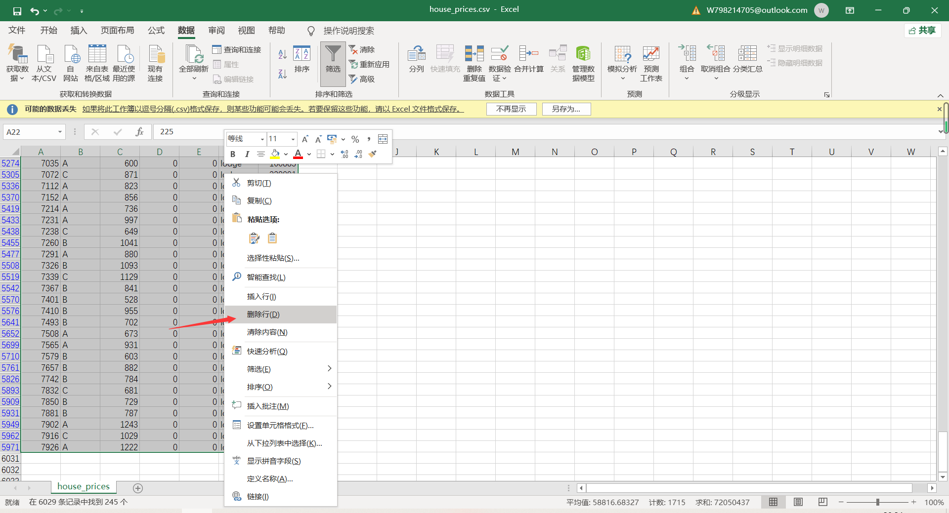
4. Deletion of missing values
(2) Non numeric data conversion
In the original data, neighborhood and style are non numeric data. It needs to be converted into numerical data before regression analysis can be carried out.
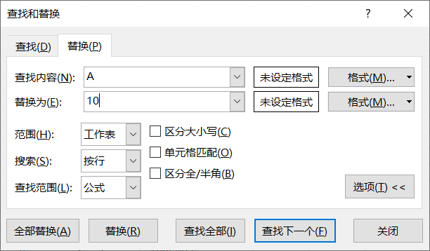
(1) Start - find and replace - replace
(2) Replace A, B and C of the original data with 10, 20 and 30, and replace victorian, ranch and lodge of the original data with 100, 200 and 300
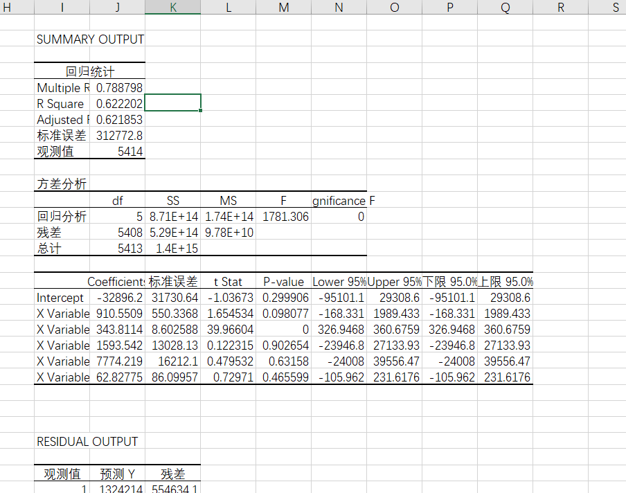
3, Excel multiple linear regression
1. Select data - data analysis - regression - determine
2. Use X and Y value interval
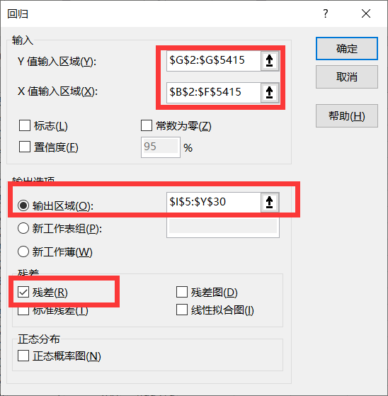
3. Results
4, Prediction of house prices by multiple linear regression model
(1) Basic package and data import
1. Import package
import pandas as pd
import numpy as np
import seaborn as sns
import matplotlib.pyplot as plt
2. Read the data from the file house_prices.csv '
df = pd.read_csv('C:/Users/86199/Jupyter/house_prices.csv')
df.info(); df.head()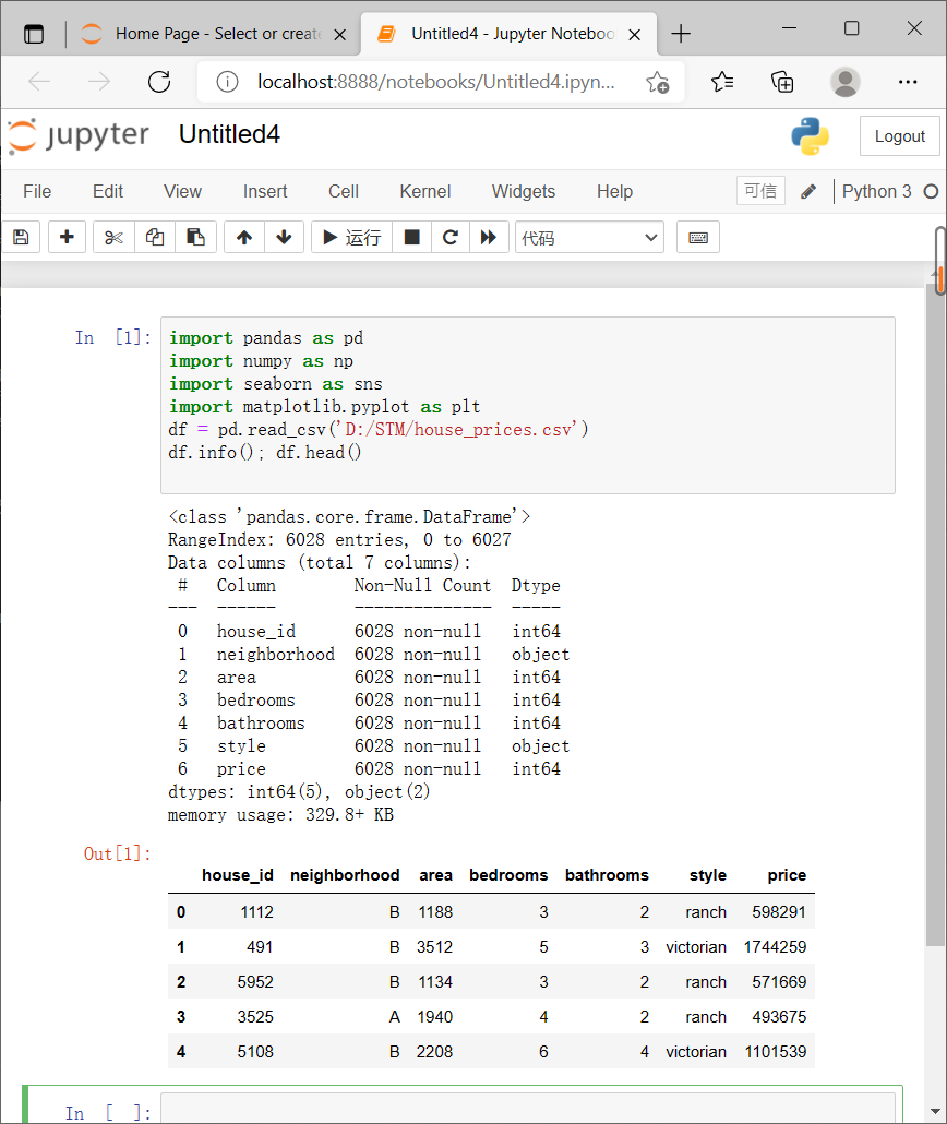
(2) Variable exploration
1. Data processing
# Outlier handling
# ================Outlier test function: two methods of IQR & Z score=========================
def outlier_test(data, column, method=None, z=2):
    """ Based on a column, the upper and lower truncation point method is used to detect outliers(Indexes) """
    """
    full_data: Complete data
    column: full_data Specified line in, format 'x' Quoted
    return Optional; outlier: Outlier data frame
    upper: Upper truncation point;  lower: Lower truncation point
    method: Method of checking outliers (optional), default None Is the upper and lower cut-off point method),
            choose Z Method, Z The default is 2
    """
    # ==================Upper and lower cut-off point method to test outliers==============================
    if method == None:
        print(f'with {column} Based on the column, the upper and lower cut-off point method is used(iqr) Detect outliers...')
        print('=' * 70)
        # Quartile; there will be exceptions when calling the function here
        column_iqr = np.quantile(data[column], 0.75) - np.quantile(data[column], 0.25)
        # 1, 3 quantiles
        (q1, q3) = np.quantile(data[column], 0.25), np.quantile(data[column], 0.75)
        # Calculate upper and lower cutoff points
        upper, lower = (q3 + 1.5 * column_iqr), (q1 - 1.5 * column_iqr)
        # Detect outliers
        outlier = data[(data[column] <= lower) | (data[column] >= upper)]
        print(f'First quantile: {q1}, Third quantile:{q3}, Interquartile range:{column_iqr}')
        print(f"Upper cutoff point:{upper}, Lower cutoff point:{lower}")
        return outlier, upper, lower
    # =====================Z-score test outliers==========================
    if method == 'z':
        """ Based on a column, the incoming data is the same as the data you want to segment z Score point, return the outlier index and the data frame """
        """
        params
        data: Complete data
        column: Specified detection column
        z: Z Quantile, The default is 2, according to z fraction-According to the normal curve table, take 2 at the left and right ends%,
           According to you z The positive and negative setting of the score. It can also be changed arbitrarily to know the data set of any top percentage
        """
        print(f'with {column} List as basis, use Z Fractional method, z Quantile extraction {z} To detect outliers...')
        print('=' * 70)
        # Calculate the numerical points of the two Z fractions
        mean, std = np.mean(data[column]), np.std(data[column])
        upper, lower = (mean + z * std), (mean - z * std)
        print(f"take {z} individual Z Score: greater than {upper} Or less than {lower} Is considered an outlier.")
        print('=' * 70)
        # Detect outliers
        outlier = data[(data[column] <= lower) | (data[column] >= upper)]
        return outlier, upper, lower
2. Call function
outlier, upper, lower = outlier_test(data=df, column='price', method='z')
outlier.info(); outlier.sample(5)
3. Delete error data
#Simply discard it here
df.drop(index=outlier.index, inplace=True)
(3) Analysis data
1. Define variables
# Category variables, also known as nominal variables
nominal_vars = ['neighborhood', 'style']

for each in nominal_vars:
    print(each, ':')
    print(df[each].agg(['value_counts']).T)
    # Direct. value_counts().T cannot achieve the following effect
     ## You must get agg, and the brackets [] inside can't be less
    print('='*35)
    # It is found that the number of each category is also OK, so as to prepare for the following analysis of variance
2. Check the correlation of variables in the thermodynamic diagram
# Thermodynamic diagram
def heatmap(data, method='pearson', camp='RdYlGn', figsize=(10 ,8)):
    """
    data: Whole data
    method: Default to pearson coefficient
    camp: The default is: RdYlGn-Red, yellow and blue; YlGnBu-Yellow green blue; Blues/Greens It's also a good choice
    figsize: The default is 10, 8
    """
    ## Eliminate color blocks with diagonal color duplication
    #     mask = np.zeros_like(df2.corr())
    #     mask[np.tril_indices_from(mask)] = True
    plt.figure(figsize=figsize, dpi= 80)
    sns.heatmap(data.corr(method=method), \
                xticklabels=data.corr(method=method).columns, \
                yticklabels=data.corr(method=method).columns, cmap=camp, \
                center=0, annot=True)
    # To achieve the effect of leaving only half of the diagonal, the parameters in brackets can be added with mask=mask
3. Call the function to output the result
# It can be seen from the thermodynamic diagram that the relationship between variables such as area, bedrooms and bathrooms and house price is still relatively strong
 ## Therefore, it is worth putting into the model, but the relationship between the classification variables style and neighborhood and price is unknown
heatmap(data=df, figsize=(6,5))

(4) Fit
1. Introduce model
(1) In the exploration just now, we found that the categories of style and neighborhood are three categories. If there are only two categories, we can conduct chi square test, so here we use analysis of variance
(2) 600 samples were randomly selected from the dataset
df = df.copy().sample(600)
# C means to tell python that this is a classified variable, otherwise Python will use it as a continuous variable
## Here, analysis of variance is directly used to test all classified variables
## The following lines of code are the standard gestures for analysis of variance using the statistical library
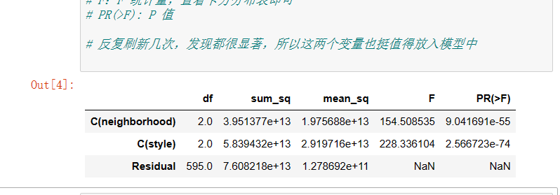
lm = ols('price ~ C(neighborhood) + C(style)', data=df).fit()
anova_lm(lm)
# The Residual line indicates the within group that cannot be explained by the model, and the others are between groups that can be explained
# df: degree of freedom (n-1) - the number of categories in the classification variable minus 1
# sum_sq: sum of squares (SSM), sum_eq: SSE of residual line
# Mean_sq: MSM, mean_sq: mse of residual line
# F: F statistics, just check the chi square distribution table
# Pr (> F): P value
# Refresh several times and find that they are very significant, so these two variables are also worth putting into the model
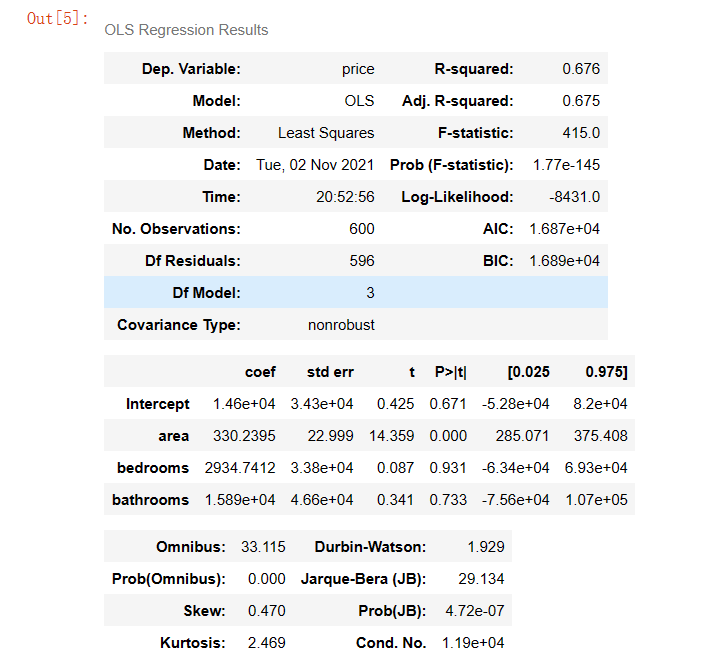
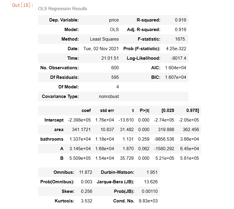
2. Multiple linear regression modeling
from statsmodels.formula.api import ols

lm = ols('price ~ area + bedrooms + bathrooms', data=df).fit()
lm.summary()
3. Model optimization
(1) It is found that the accuracy is not high enough. Here, the accuracy of the model is improved by adding dummy variables and using variance expansion factor to detect multicollinearity
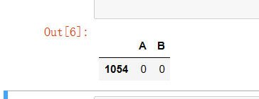
# Set dummy variable
# Take the nominal variable neighborhood as an example
nominal_data = df['neighborhood']

# Set dummy variable
dummies = pd.get_dummies(nominal_data)
dummies.sample()  # pandas will automatically name it for you

# One dummy variable generated by each nominal variable needs to be discarded. Here, take discarding C as an example
dummies.drop(columns=['C'], inplace=True)
dummies.sample()
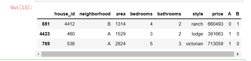
(2) The results are spliced with the original data set
# Splice the results with the original data set
results = pd.concat(objs=[df, dummies], axis='columns')  # Merge by column
results.sample(3)
# You can try to handle the nominal variable style by yourself
4. Modeling again
(1) Code
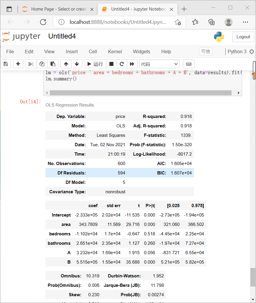
# Modeling again
lm = ols('price ~ area + bedrooms + bathrooms + A + B', data=results).fit()
lm.summary()
5. Deal with Multicollinearity
(1) # user defined variance expansion factor detection formula
def vif(df, col_i):
    """
    df: Whole data
    col_i: Detected column name
    """
    cols = list(df.columns)
    cols.remove(col_i)
    cols_noti = cols
    formula = col_i + '~' + '+'.join(cols_noti)
    r2 = ols(formula, df).fit().rsquared
    return 1. / (1. - r2)
(2) Function call
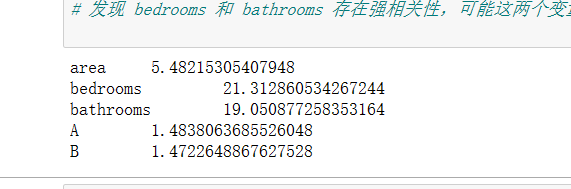
test_data = results[['area', 'bedrooms', 'bathrooms', 'A', 'B']]
for i in test_data.columns:
    print(i, '\t', vif(df=test_data, col_i=i))
# It is found that there is a strong correlation between bedrooms and bathrooms, which may explain the same problem
6. Fit again
lm = ols(formula='price ~ area + bathrooms + A + B', data=results).fit()
lm.summary()
(3) There is still multicollinearity. Test again
test_data = df[['area', 'bathrooms']]
for i in test_data.columns:
    print(i, '\t', vif(df=test_data, col_i=i))
4, Prediction of house prices by multiple linear regression of sklearn
(1) No data processing
1. Import package and data
import pandas as pd
import numpy as np
import math
import matplotlib.pyplot as plt # Drawing
from sklearn import linear_model # linear model
data = pd.read_csv('D:/Users/86199/Jupyter/house_prices_second.csv') #Read data
data.head() #Data display
2. Remove the first column of house_id
new_data=data.iloc[:,1:] #Get rid of the id column
new_data.head()
3. Relationship coefficient matrix display
new_data.corr() # Correlation coefficient matrix, only statistical value column
4. Assignment variable
x_data = new_data.iloc[:, 0:5] #Corresponding columns of area, bedrooms and bathroom
y_data = new_data.iloc[:, -1] #price corresponding column
print(x_data, y_data, len(x_data))
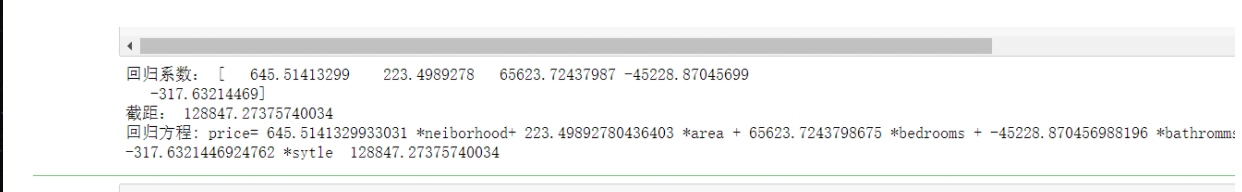
5. Establish the model and output the results
# Application model
model = linear_model.LinearRegression()
model.fit(x_data, y_data)
print("Regression coefficient:", model.coef_)
print("Intercept:", model.intercept_)
print('regression equation : price=',model.coef_[0],'*neiborhood+',model.coef_[1],'*area +',model.coef_[2],'*bedrooms +',model.coef_[3],'*bathromms +',model.coef_[4],'*sytle ',model.intercept_)
(2) The data shall be cleaned before solving
1. Assign a new variable
new_data_Z=new_data.iloc[:,0:]
new_data_IQR=new_data.iloc[:,0:]
2. Abnormal value handling
# ================Outlier test function: two methods of IQR & Z score=========================
def outlier_test(data, column, method=None, z=2):
    """ Based on a column, the upper and lower truncation point method is used to detect outliers(Indexes) """
    """
    full_data: Complete data
    column: full_data Specified line in, format 'x' Quoted
    return Optional; outlier: Outlier data frame
    upper: Upper truncation point;  lower: Lower truncation point
    method: Method of checking outliers (optional), default None Is the upper and lower cut-off point method),
            choose Z Method, Z The default is 2
    """
    # ==================Upper and lower cut-off point method to test outliers==============================
    if method == None:
        print(f'with {column} Based on the column, the upper and lower cut-off point method is used(iqr) Detect outliers...')
        print('=' * 70)
        # Quartile; There will be exceptions when calling the function here
        column_iqr = np.quantile(data[column], 0.75) - np.quantile(data[column], 0.25)
        # 1, 3 quantiles
        (q1, q3) = np.quantile(data[column], 0.25), np.quantile(data[column], 0.75)
        # Calculate upper and lower cutoff points
        upper, lower = (q3 + 1.5 * column_iqr), (q1 - 1.5 * column_iqr)
        # Detect outliers
        outlier = data[(data[column] <= lower) | (data[column] >= upper)]
        print(f'First quantile: {q1}, Third quantile:{q3}, Interquartile range:{column_iqr}')
        print(f"Upper cutoff point:{upper}, Lower cutoff point:{lower}")
        return outlier, upper, lower
    # =====================Z-score test outliers==========================
    if method == 'z':
        """ Based on a column, the incoming data is the same as the data you want to segment z Score point, return the outlier index and the data frame """
        """
        params
        data: Complete data
        column: Specified detection column
        z: Z Quantile, The default is 2, according to z fraction-According to the normal curve table, take 2 at the left and right ends%,
           According to you z Positive and negative setting of scores. It can also be changed arbitrarily to know the data set of any top percentage
        """
        print(f'with {column} List as basis, use Z Fractional method, z Quantile extraction {z} To detect outliers...')
        print('=' * 70)
        # Calculate the numerical points of the two Z fractions
        mean, std = np.mean(data[column]), np.std(data[column])
        upper, lower = (mean + z * std), (mean - z * std)
        print(f"take {z} individual Z Score: greater than {upper} Or less than {lower} Is considered an outlier.")
        print('=' * 70)
        # Detect outliers
        outlier = data[(data[column] <= lower) | (data[column] >= upper)]
        return outlier, upper, lower
3. Based on the price column, the Z-score method is used, and the z-quantile is taken as 2 to detect abnormal values
outlier, upper, lower = outlier_test(data=new_data_Z, column='price', method='z')
outlier.info(); outlier.sample(5)

# Simply discard it here
new_data_Z.drop(index=outlier.index, inplace=True)
4. Based on the price column, the upper and lower cut-off point method (iqr) is used to detect abnormal values
outlier, upper, lower = outlier_test(data=new_data_IQR, column='price')
outlier.info(); outlier.sample(6)

# Simply discard it here
new_data_IQR.drop(index=outlier.index, inplace=True)
5. Output original data correlation matrix
print("Original data correlation matrix")
new_data.corr()
6. Data correlation matrix processed by Z method
Insert the code slice here print("Z Data correlation matrix processed by method")
new_data_Z.corr()
7. Data correlation matrix processed by IQR method
print("IQR Data correlation matrix processed by method")
new_data_IQR.corr()
8. Modeling output
x_data = new_data_Z.iloc[:, 0:5]
y_data = new_data_Z.iloc[:, -1]
# Application model
model = linear_model.LinearRegression()
model.fit(x_data, y_data)
print("Regression coefficient:", model.coef_)
print("Intercept:", model.intercept_)
print('regression equation : price=',model.coef_[0],'*neiborhood+',model.coef_[1],'*area +',model.coef_[2],'*bedrooms +',model.coef_[3],'*bathromms +',model.coef_[4],'*sytle ',model.intercept_)
5, Summary
This experiment understands the related concepts of multiple regression model and the basic steps of constructing the model. Learned how to use Excel table to build multiple regression model. In fact, the methods used in univariate linear regression are very similar. The only difference is the selection of X-value interval, which changes from single variable to multiple variables in univariate linear regression. Be more familiar with the method of calling functions using sklearn library, and understand some basic methods of processing data, including processing default values and non numerical data.