Introduction

With the increasing complexity and diversity of cloud computing network environment, the problem of occasional network jitter has become a major problem for cloud services. However, when dealing with such problems, the traditional network performance tools (sar, ss, tcpdump, etc.) based on kernel internal statistics and network packet capture are limited, and the tracking tools developed based on BPF can play a good complementary role. BPF's powerful system level observation ability, deeper and more detailed auxiliary performance analysis and problem location are especially suitable for solving the problem of occasional network jitter. Starting with a practical business case, this paper introduces how to locate and solve the problem of request timeout and network jitter with one in millions probability based on BPF tracking technology, hoping to inspire interested readers.

Problem background

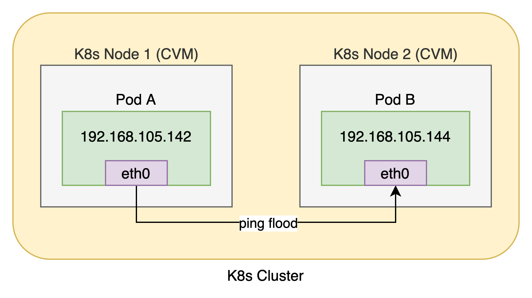
According to the feedback from the business party, a delay sensitive application began to experience occasional request timeout since it was migrated to the container cloud platform (never before migration). In view of this phenomenon, we ping flood the network of the container cloud platform in the test environment under the same conditions to observe whether the network jitter can be reproduced. The specific scenario of ping flood is shown in the figure below. Pod A and Pod B are in the same K8s cluster. Pod a initiates ping flood to Pod B, with a total of 50 million ping requests.

The ping flood results show that the average ping request delay is 0.058 ms, a total of 10 ~ 20 times, more than 1 ms. the Debug information is shown below.

# ping -D -f 192.168.105.144

PING 192.168.105.144 (192.168.105.144) 56(84) bytes of data.
[1633177499.852333]  icmp_seq=58063 time=1.30 ms
[1633177506.879423]  icmp_seq=21613 time=1.27 ms
[1633177522.629392]  icmp_seq=36949 time=1.29 ms
[1633177580.466357]  icmp_seq=28338 time=2.37 ms
[1633177680.083396]  icmp_seq=55992 time=1.27 ms
...

rtt min/avg/max/mdev = 0.034/0.058/2.376/0.006 ms, ipg/ewma 0.073/0.046 ms

Repeated execution for several times shows basically the same performance, which is equivalent to stably reproducing the network jitter problem of the production environment.

Next, this paper will further analyze the occasional network jitter of ping flood. Firstly, write a new BPF tracking tool to analyze the processing of ping requests in the network protocol stack and find key clues, then use the existing BPF tracking tool to locate the root cause, and finally propose a compromise solution to eliminate the network jitter problem in the production environment of container cloud platform.

problem analysis

At the beginning, we first used traditional performance tools (top, free, sar, iostat, etc.) for qualitative analysis, and found that there were no obvious abnormalities in CPU utilization, average load, memory, network traffic, packet loss, disk I/O and other indicators. The difficulty of analyzing the network jitter problem lies in the contingency. When the jitter really occurs, there is a lack of detailed on-site state information. The traditional performance tools are a little stretched to deal with this kind of problem, and the tracking tool based on BPF can make up for this defect. BPF's powerful system level observation ability, deeper and more detailed auxiliary performance analysis and problem location are especially suitable for solving the problem of occasional network jitter. Therefore, we began to try to analyze the problem based on BPF.

Reasons for BPF selection

• Traditional network performance tools can display various statistical information in the kernel, including packet rate, throughput, socket status and so on. However, the kernel state is the blind spot of these tools. They can't see which data packets are sent by which process, the corresponding call stack information and the kernel state of socket and TCP. This information can only be obtained with the help of BPF tracking tools or lower level Tracepoints and kprobes.
• The minimum statistical interval of most traditional network performance tools is in seconds, so it is difficult to identify ping requests with a maximum delay of only a few ms.
• The common network packet capturing tool tcpdump not only increases the processing overhead of each network packet, but also increases the CPU, memory and storage overhead when writing packets to the file system, but also the overhead when reading and processing in the later stage. In contrast, using BPF to track each network packet itself improves efficiency a lot. Because BPF directly saves statistics in kernel memory without capturing package files. BPF uses Tracepoints and kprobes to explore the internal situation of network software stack, expand the network observability provided by traditional network performance tools, and provide more new ideas for fine-grained analysis of network problems.

BPF tool design ideas

At present, there is no ready-made BPF tool that can provide fine-grained ping packet tracking, but we can easily write custom BPF tools using BPF front-end bcc.

For the sending and receiving process of ping packets, we have compiled BPF tools pingsnd and pingrcv tracking tools. The general design idea is as follows:

• kprobes is used to record the status information, time consumption and time difference between the key functions (napi_gro_receive, _netif_receive_skb_core, virtqueue_xxx, etc.) of ping packets at the sending end and receiving end of the network software stack, so as to analyze the delay of the processing flow of the network software stack. The key functions are shown in the figure below, in which the solid arrow identifies the ping request processing process and the dotted arrow identifies the ping reply processing process, which together constitute a complete ping request.

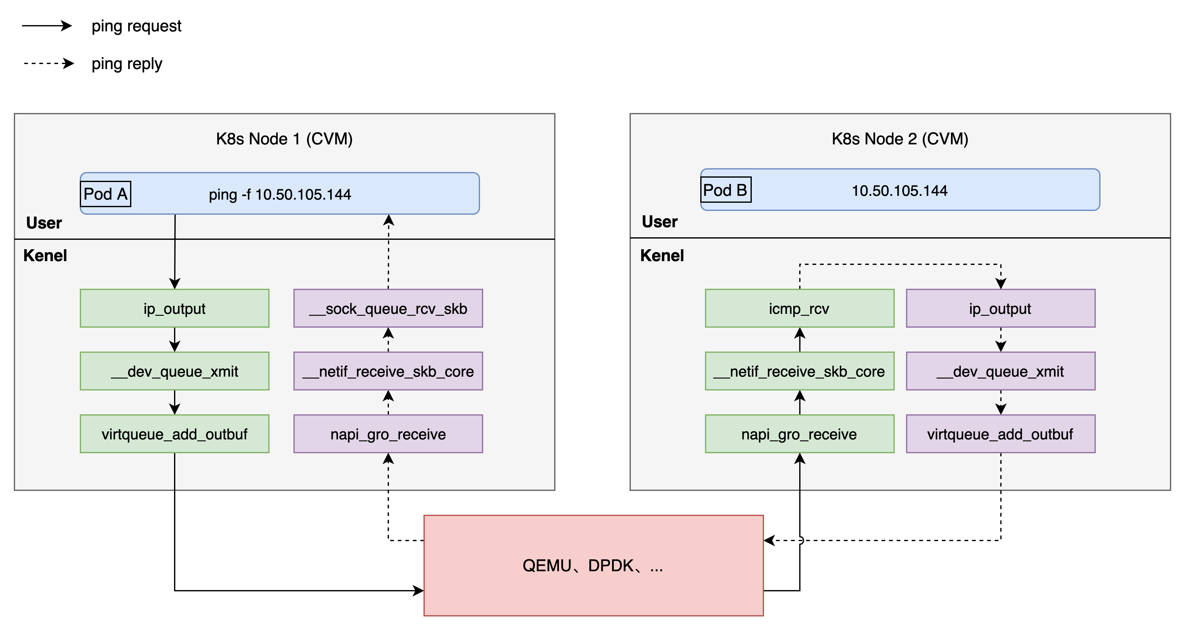
• ping sending end and receiving end are tracked separately, and finally corresponding pingsnd and pingrcv tracking tools are formed. Pingsnd and pingrcv tracking tools record context information such as CPU number, process name and system time with ICMP number as the primary key every time an event occurs.
• pingsnd only tracks packets related to the specified destination IP address, and filters packets whose processing time at the sending end of ping is less than the specified minimum threshold (the default minimum threshold is 0 ms, and filtering is not performed).
• pingrcv only tracks the packets related to the specified source IP address, and filters the packets whose processing time at the ping receiving end is less than the specified minimum threshold (the default minimum threshold is 0 ms, and filtering is not performed).

BPF tool test ox knife

1. The ping sending end (Pod A) executes pingsnd, and the tracking destination IP is 192.168.105.144 (Pod B) for all ping requests.

(Pod A)# ./pingsnd -i 192.168.105.144 > /run/pingsnd.log

When the tracking results are written to the tmpfs file, ext4fs may be too late to write, resulting in the loss of some tracking events.

2. ping receiver (Pod B) executes pingrcv to track all ping requests:

(Pod B)# ./pingrcv -i 192.168.105.144 > /run/pingrcv.log

When the tracking results are written to the tmpfs file, ext4fs may be too late to write, resulting in the loss of some tracking events.

3. Execute the ping flood command:

(Pod A)# ping -f -D 192.168.105.144

4. After running for a period of time, there are 5 ping requests greater than 1ms in total (covering the two types of situations to be analyzed). Next, these requests will be used as analysis samples. For ease of expression, they are numbered pr1, pr2, pr3, pr4 and pr5 respectively.

PING 192.168.105.144 (192.168.105.144) 56(84) bytes of data.
[1633177499.852333]  icmp_seq=58063 time=1.30 ms
[1633177506.879423]  icmp_seq=21613 time=1.27 ms
[1633177522.629392]  icmp_seq=36949 time=1.29 ms
[1633177580.466357]  icmp_seq=28338 time=1.29 ms
[1633177680.083396]  icmp_seq=55992 time=1.27 ms

--- 192.168.105.144 ping statistics ---
3329313 packets transmitted, 3329083 received, 0% packet loss, time 243393ms
rtt min/avg/max/mdev = 0.034/0.058/1.306/0.006 ms, ipg/ewma 0.073/0.046 ms

5 first analyze pr1 (icmp_seq: 58063) according to timestamp and ICMP_ Seq, search the tracking result file / run/pingsnd.log in step 1. The tracking results of pr1 at the sending end are as follows.

2021-10-02 20:24:59.736836
1. send ping at ip_output                  seq:58063 cpu:7  pid:579577   delta(ms):0.000
2. send ping at __dev_queue_xmit           seq:58063 cpu:7  pid:579577   delta(ms):0.001
3. send ping at virtqueue_add_outbuf       seq:58063 cpu:7  pid:579577   delta(ms):0.002
4. recv ping at napi_gro_receive           seq:58063 cpu:10 pid:0        delta(ms):1.304
5. recv ping at __netif_receive_skb_core   seq:58063 cpu:7  pid:0        delta(ms):1.309
6. recv ping at __sock_queue_rcv_skb       seq:58063 cpu:7  pid:0        delta(ms):1.310

1 ~ 3 add the ping request packet to the vring queue. 3 ~ 4 time difference is greater than 1ms. 4 ~ 6 receive the ping reply packet in the network protocol stack and deliver it to the socket receiving queue. The processing time of network protocol stack accounts for a small proportion. 4 is executed on CPU 10 and 5 is executed on CPU 7. RPS load balancing actually occurs behind it. (this is also the case with the following tracking results, which will not be repeated one by one.)

Search the tracking result file / run/pingrcv.log in step 2. The tracking results of pr1 (icmp_seq: 58063) at the receiving end are as follows.

2021-10-02 20:24:58.895722
1. recv ping at napi_gro_receive           seq:58063 cpu:15 pid:100      delta(ms):0.000
2. recv ping at __netif_receive_skb_core   seq:58063 cpu:15 pid:100      delta(ms):0.001
3. recv ping at icmp_recv                  seq:58063 cpu:9  pid:0        delta(ms):0.011
4. send ping at ip_output                  seq:58063 cpu:9  pid:0        delta(ms):0.012
5. send ping at __dev_queue_xmit           seq:58063 cpu:9  pid:0        delta(ms):0.013
6. send ping at virtqueue_add_outbuf       seq:58063 cpu:9  pid:0        delta(ms):0.014

The ping request packet is received in the 1 ~ 3 network protocol stack and processed by the kernel thread Ksoft irqd / 15 (PID: 100) running on CPU 15. The processing time of network protocol stack is small (0.014 ms). 4 ~ 6 add the ping request packet to the vring queue.

6 similarly, the tracking results of pr2 (icmp_seq: 21613) at the transmitter are as follows.

2021-10-02 20:25:06.763924
1. send ping at ip_output                  seq:21613 cpu:7  pid:579577   delta(ms):0.000
2. send ping at __dev_queue_xmit           seq:21613 cpu:7  pid:579577   delta(ms):0.001
3. send ping at virtqueue_add_outbuf       seq:21613 cpu:7  pid:579577   delta(ms):0.002
4. recv ping at napi_gro_receive           seq:21613 cpu:10 pid:70       delta(ms):1.271
5. recv ping at __netif_receive_skb_core   seq:21613 cpu:7  pid:0        delta(ms):1.275
6. recv ping at __sock_queue_rcv_skb       seq:21613 cpu:7  pid:0        delta(ms):1.285

1 ~ 3 add the ping request packet to the vring queue. 3 ~ 4 time difference is greater than 1ms. Where NaPi_ gro_ The receive is triggered by the kernel thread ksoftirqd/10 (pid: 70) running on CPU 10. 4 ~ 6 receive the ping reply packet in the network protocol stack and deliver it to the socket receiving queue. The processing time of network protocol stack is small (0.016ms).

The tracking results of pr2 (icmp_seq: 21613) at the receiving end are as follows.

2021-10-02 20:25:05.921582
1. recv ping at napi_gro_receive           seq:21613 cpu:15 pid:0        delta(ms):0.000
2. recv ping at __netif_receive_skb_core   seq:21613 cpu:15 pid:0        delta(ms):0.005
3. recv ping at icmp_recv                  seq:21613 cpu:9  pid:0        delta(ms):0.006
4. send ping at ip_output                  seq:21613 cpu:9  pid:0        delta(ms):0.007
5. send ping at __dev_queue_xmit           seq:21613 cpu:9  pid:0        delta(ms):0.007
6. send ping at virtqueue_add_outbuf       seq:21613 cpu:9  pid:0        delta(ms):0.008

1 ~ 3 receive the ping request packet in the network protocol stack. 4 ~ 6 add the ping request packet to the vring queue. The processing time of network protocol stack is small (0.008 ms).

7 continue to analyze pr3 ~ pr5 in turn. The results show that when the ping request is delayed and jittered, the processing time of the network protocol stack accounts for a small proportion. BPF tools such as pingsnd and pindrcv do not clearly locate the specific location where a large proportion of delay occurs. However, it provides a valuable clue: ping the key function NaPi for packet reception_ gro_ Receive is triggered by the kernel thread ksoftirqd/xx. The statistics of pr1 ~ pr5 are shown in the table below. Therefore, it is preliminarily suspected that the network jitter is caused by the scheduling delay of soft interrupt thread ksoftirqd/xx.

8 in order to verify this idea, execute the existing BCC tool runqslower at the ping sending end and receiving end respectively to track scheduling delay events greater than 1000 ms. here, only focus on ksoftirqd kernel threads. The specific commands are as follows:

# ./runqslower 1000 | grep ksoftirqd

Perf sched can also be used to analyze task scheduling delays. However, compared with the existing BPF tools runqlat and runqslower, the overhead is very large (including event data copy, disk I/O, subsequent analysis and statistics overhead, etc.), especially in very busy production systems. Therefore, perf sched is not recommended when BPF tools are available.

Then, the ping sender executes ping flood. After a period of time, the following ping requests greater than 1ms (5 times in total).

[1634029324.545499]  icmp_seq=16704 time=1.52 ms
[1634029414.366726]  icmp_seq=55064 time=1.40 ms
[1634029414.780387]  icmp_seq=61242 time=1.44 ms
[1634029469.778275]  icmp_seq=35284 time=1.37 ms
[1634029714.109554]  icmp_seq=34807 time=2.48 ms

Check the ping sender tracking results twice in total, which coincides with the time points of two requests of the above ping flood output results.

# ./runqslower 1000 | grep ksoftirqd

Tracing run queue latency higher than 1000 us
TIME     COMM             PID           LAT(us)
17:04:29 ksoftirqd/15     100              1372
17:08:34 ksoftirqd/15     100              2482

Check the ping receiver tracking results for three times, which coincides with the time points of three requests of the above ping flood output results.

# ./runqslower 1000 | grep ksoftirqd

Tracing run queue latency higher than 1000 us
TIME     COMM             PID           LAT(us)
17:02:04 ksoftirqd/6      46               1509
17:03:34 ksoftirqd/7      52               1346
17:03:34 ksoftirqd/7      52               1372

The sending end and receiving end of the ping have tracked the ksoftirqd/xx soft interrupt scheduling delay greater than 1ms for five times, which is consistent with the occurrence time of each ping request in the above ping flood output results.

The existing BCC tool runqlat is convenient to view the scheduling delay distribution histogram of the whole or specified process. It can also find the above ksoftirqd/xx soft interrupt scheduling delay problem. Interested readers can try it.

9 (optional reading) with the help of pingsnd and pingrcv tracking tools, the specific location of delay jitter is not directly found. We can continue to expand its boundary and further refine the key links of ping requests. The whole process is relatively complex. I won't expand it in detail here. Let's talk about the idea roughly. I wrote a BCC tool vring for this purpose_ Interrupt is used to track the time point of the last vring_interrupt of the received packet event (napi_gro_receive) and try to analyze vring_ interrupt -> napi_ gro_ Whether there is a large time difference between receives. vring_ The interrupt parameter does not contain skb, so it cannot be directly aligned with the time points of events related to pingsnd and pingrcv. However, when the Pod network card does not ping flood, there are basically no data packets (occasionally a very small number of IGMP data packets), so it provides computing vring_ interrupt -> napi_ gro_ Possibility of receiving time difference. When vring_ When the interrupt event occurs, filter according to the irq number (for example, the irq range of eth0 network card queue in Pod B is 45 ~ 52), and then print the CPU, process name, process ID and timestamp corresponding to the time of the event. Finally, the scheduling delay of Ksoft irqd kernel thread can be indirectly analyzed by combining the output of pingsnd and pingrcv tracking tools.

Using the newly compiled vring_interrupt tool, combined with pingsnd and pingrcv, analyzes the specific location of delay jitter in vring_interrupt -> napi_ gro_ Between receive.

Optimization scheme

For Ksoft irqd soft interrupt scheduling delay, a common compromise solution is to change the scheduling policy and optimization level of Ksoft irqd kernel threads, such as modifying the scheduling policy to real-time scheduling RR or FIFO. The scheme also has side effects and is not universal, but it is applicable to delay sensitive applications to some extent. In fact, Linux soft interrupt processing itself is full of many compromise logic and is still improving.

Since the scheduling delay of Ksoft irqd soft interrupt may exist at both the sending and receiving ends of ping, both ends need to modify the scheduling strategy and optimization level of Ksoft irqd kernel threads.

pgrep ksoftirqd | xargs -t -n1 chrt -r -p 99

It is recommended to obtain the list of Pod network card queue irq bound CPU s, and only modify the scheduling policy and optimization level of ksoftirqd kernel threads corresponding to the list.

Implement the compromise scheme, then execute ping flood, and there will be no more ping requests greater than 1ms.

Better solutions need to be further explored...

Summary thinking

In view of the above network jitter problem, we have compiled BPF tools pingsnd and pingrcv, combined with the existing BPF tools runqlat and runqslower, and located that Ksoft irqd soft interrupt scheduling delay is the culprit of the network jitter problem. Finally, an optimization scheme is proposed to solve the low probability network jitter problem.

• Compared with traditional tools, BCC tool greatly improves the system observation ability and is suitable for analyzing network jitter, scheduler delay and other problems. However, do not trust the tool itself too much. When the results do not meet expectations, remain skeptical. In this process, many BCC tools have been stepped on, including softirqs, runqlat and runqlower, which have small problems in the existing environment.
• When the existing tools of BPF are not enough, try to create tools to provide more fine-grained downhole analysis capability.

BPF common tools appendix

The BPF tools used in troubleshooting the problem are summarized as follows for readers' reference.

# Check the trigger frequency and cumulative time of hard interrupt
/usr/share/bcc/tools/hardirqs -C 1
/usr/share/bcc/tools/hardirqs -d -NT 1

# View soft interrupt delay distribution, cumulative time consumption, etc
/usr/share/bcc/tools/softirqs 1 10
/usr/share/bcc/tools/softirqs -dT 1

# Specify CPU, sampling frequency (more efficient than perf record):
/usr/share/bcc/tools/profile -f -C 14 -F 999

# Count of kernel functions such as network packet reception and RPS
/usr/share/bcc/tools/funccount -i 1 napi_gro_receive
/usr/share/bcc/tools/funccount -i 1 get_rps_cpu

# To view kernel function delay distribution:
/usr/share/bcc/tools/funclatency -uTi 5 __do_softirq
/usr/share/bcc/tools/funclatency -uTi 5 net_rx_action

# View kernel function parameter distribution and call times:
/usr/share/bcc/tools/argdist -H 'r::vfs_read()'
/usr/share/bcc/tools/argdist -C 'r::vfs_read()'
/usr/share/bcc/tools/argdist -H 't:net:net_dev_queue():u32:args->len'

# Track the status information of each occurrence of the event
/usr/share/bcc/tools/trace -C 'r::vfs_read "%d", retval'

# View the scheduling delay of the specified thread:
/usr/share/bcc/tools/runqlat 1 10
/usr/share/bcc/tools/runqlat -p 94 -mT 2

# View scheduling delays greater than the specified duration:
/usr/share/bcc/tools/runqslower 1000
/usr/share/bcc/tools/runqslower -p 94 1000

# View stack + count:
/usr/share/bcc/tools/stackcount -Ti 5 icmp_rcv
/usr/share/bcc/tools/stackcount -Ti 5 vring_interrupt
/usr/share/bcc/tools/stackcount -c 12 -i 1 __raise_softirq_irqoff

This article refers to the operational requirements of BPF tools

1. Required kernel version: 4.9+
2. BCC pre-installed: yum -y install bcc