What is polynomial regression

The idea of polynomial regression is similar to that of multivariate linear regression. It only adds new features to the original data samples, and the new features are the combination of polynomials of the original features. In the case that linear regression can not fit the existing data well, it is possible that the curve obtained after a feature is square or cubic can fit the data well. This regression method is called polynomial regression.

Polynomial Regression and pipeline in Sckit-Learn

import numpy as np
from sklearn.preprocessing import PolynomialFeatures
from sklearn.linear_model import LinearRegression
from sklearn.pipeline import Pipeline
from sklearn.preprocessing import StandardScaler

# Analog data set
x = np.random.uniform(-2, 3, size=100)
X = x.reshape(-1, 1)
y = 0.5 * x**2 + x + 2 + np.random.normal(0, 1, 100)

# Add features to the data set (there is only one original feature)
poly = PolynomialFeatures(degree=2)
poly.fit(X)
X2 = poly.transform(X)
print(X2.shape)

# Prediction by Linear Regression
lin_reg = LinearRegression()
lin_reg.fit(X2, y)
y_predict = lin_reg.predict(X2)
print(lin_reg.coef_)

# Using pipeline
poly_reg = Pipeline([
    ('poly', PolynomialFeatures(degree=2)),
    ('std_scaler', StandardScaler()),
    ('lin_reg', LinearRegression())
])

poly_reg.fit(X, y)
y_predict = poly_reg.predict(X)

Overfitting and Unfitting

Overfitting refers to the excessive fitting degree of training data by the model.

When a model excessively learns the details and noises in the training data, so that the model performs poorly on the new data, we call it fitting. This means that noise or random fluctuations in training data are also learned as concepts by the model. The problem is that these concepts do not apply to new data, resulting in poor generalization performance of models.

Overfitting is more likely to occur in parametric non-linear models, because the process of learning objective functions is variable and elastic. Similarly, many parametric-free learning algorithms also include parameters or techniques that limit the number of concepts learned by constrained models.

Unfitting refers to the poor performance of models in training and prediction.

An under-fitting machine learning model is not a good model and it is obvious that it does not perform well in training data.

Underfitting is usually not discussed, because given an index for evaluating the performance of a model, underfitting can easily be found. The correction method is to continue learning and try to replace machine learning algorithms. Nevertheless, there is a sharp contrast between under-fitting and over-fitting.

Why Training Data Set and Test Data Set

The solution of over-fitting is to use training data set and test data set to select the model.
Even if the training data set is used for model training, we choose the model with smaller error on the test data set, rather than the model with better fitting to the training data set. The prediction ability of the model on the test data set is called generalization ability.
The relationship between model accuracy and model complexity:

In fact, this is a process from under-fitting to over-fitting as the complexity of the model increases. The main task of machine learning is to find the best generalization ability.

learning curve

Over-fitting and under-fitting from the point of view of learning curve
Learning curve: With the gradual increase of training samples, the performance of the model trained by the algorithm.
Overfitting: The error on training data sets is small, while the error on testing data sets is large.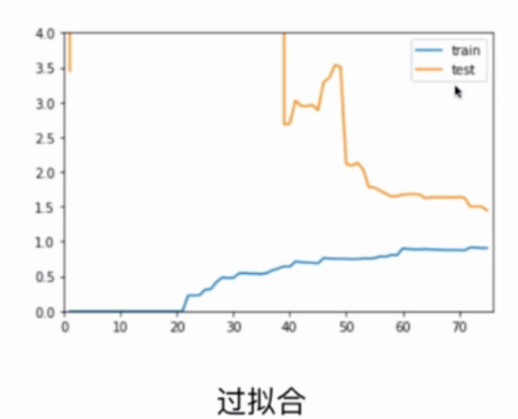

Optimum: The error of over-fitting on training data set and test data set is relatively small.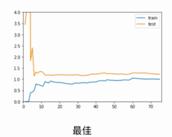

Unfitting: The error of training data set is large, and the error of testing data set is also large.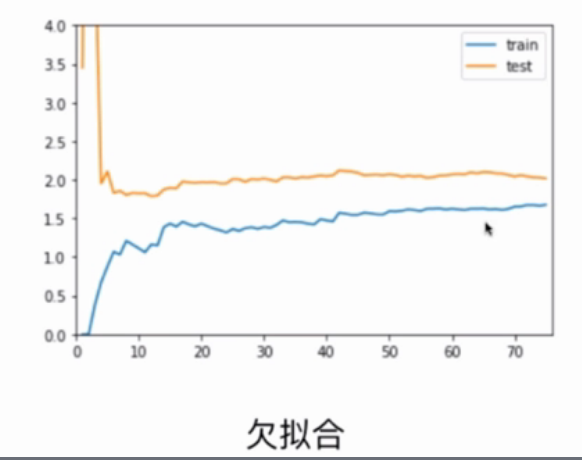

Verification Data Set and Cross-validation

When using training data and test data for model selection, because the test data set is known, our work is around adjusting parameters to make the model have good generalization ability in the test data set. The problem that may arise is that the model is over-fitting for a specific test data set.

Validation data set

The way to solve the above problems is to divide the data set into training data set (training model), validate the data set (evaluate the generalization ability of the model and adjust the hyper-parameters accordingly), and test the data set (test data in simulated real environment to measure the performance of the final model).

Cross validation

k-folds cross validation: the training data set is divided into k parts, k-1 part is the training set and 1 part is the verification set. Although the Super-parameters found by this method are more trustworthy, the disadvantage of this method is that the overall performance of training K models per time is slower than k times.
Leave-One-Out Cross Validation: The training data set (m samples) is divided into m parts, m-1 part is the training set and 1 part is the verification machine. This method is completely free from random influence and is the closest to the real performance index of the model, but it has a huge amount of calculation.
The following is cross_val_score cross-validation:

import numpy as np
from sklearn import datasets
from sklearn.model_selection import train_test_split
from sklearn.neighbors import KNeighborsClassifier
from sklearn.model_selection import cross_val_score

digits = datasets.load_digits()
X = digits.data
y = digits.target

X_train,X_test,y_train,y_test = train_test_split(X,y,test_size=0.4,random_state=666)

best_score, best_k, best_p = 0, 0, 0
for k in range(2,11):
  for p in range(1,6):
    knn_clf =  KNeighborsClassifier(weights='distance',n_neighbors=k,p=p)
    # Using cross validation
    score = cross_val_score(knn_clf,X_train,y_train)
    score = np.mean(score)
    if score > best_score:
      best_score, best_k, best_p = score, k, p
      
knn_clf2 =  KNeighborsClassifier(weights='distance',n_neighbors=best_k,p=best_p)
knn_clf2.fit(X_train,y_train)
score_test = knn_clf2.score(X_test,y_test)
print(score_test)

print('Best_k = ', best_k)
print('Best_p = ', best_p)
print('Best_score = ', best_score)

GridSearch actually includes cross-validation:

 # Grid search (including cross validation)
    from sklearn.model_selection import GridSearchCV
    import numpy as np
    from sklearn import datasets
    from sklearn.model_selection import train_test_split
    from sklearn.neighbors import KNeighborsClassifier
    
    digits = datasets.load_digits()
    X = digits.data
    y = digits.target
    
    X_train,X_test,y_train,y_test = train_test_split(X,y,test_size=0.4,random_state=666)
    
    param_grid = [
      {
      'weights': ['distance'],
      'n_neighbors':[i for i in range(2,11)],
      'p':[i for i in range(1,6)]
      }
    ]
    knn_clf =  KNeighborsClassifier()
    grid_search = GridSearchCV(knn_clf,param_grid,verbose=1)
    grid_search.fit(X_train,y_train)
    print(grid_search.best_score_)
    print(grid_search.best_params_)
    print(grid_search.best_estimator_)

Trade-off of deviation variance

From a higher perspective, we can see more comprehensively how to classify the errors in machine learning: deviation and variance.

Deviation and variance

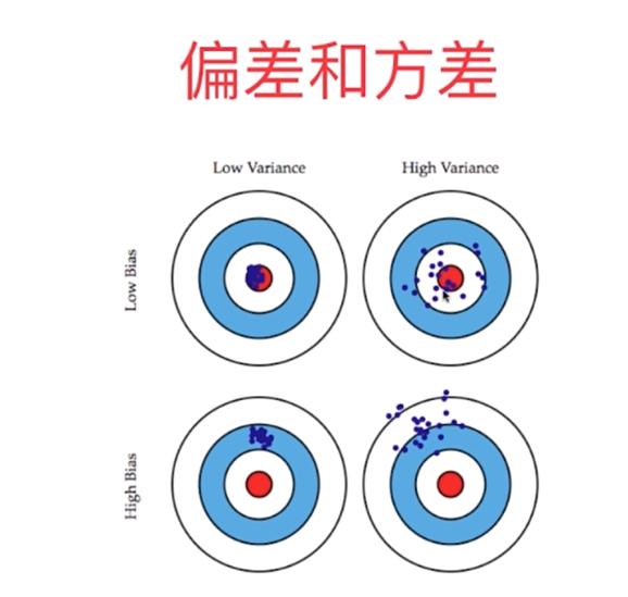
Model error = Bias + Variance + Inevitable error
The main reason for the deviation is that the assumption of the problem itself is incorrect, such as the use of linear regression for non-linear data. That is to say, underfitting.
The main reason for the variance is that the model used is too complex, such as high-order regression.
Some algorithms are inherently high variance algorithms, such as kNN. Generally speaking, non-parametric learning is usually high variance algorithms, because there is no assumption about the data.
Some algorithms are inherently high-deviation algorithms, such as linear regression. Generally speaking, parameter learning is a high-deviation algorithm because of strong assumptions about data.
Most algorithms have corresponding parameters and can adjust deviation and variance. The deviation and variance are usually contradictory, reducing the deviation will increase the variance, reducing the variance will increase the deviation, so it is necessary to weigh the deviation and variance. The main challenge of machine learning comes from variance.
Usually the means to solve high variance are:

• Reducing Model Complexity
• Reducing data dimension; Noise reduction
• Increase sample size
• Using Verification Sets
• Model regularization

Model generalization and ridge regression

Regularization of models

Model regularization: limit the size of parameters to solve the problem of model over-fitting, that is, too large variance.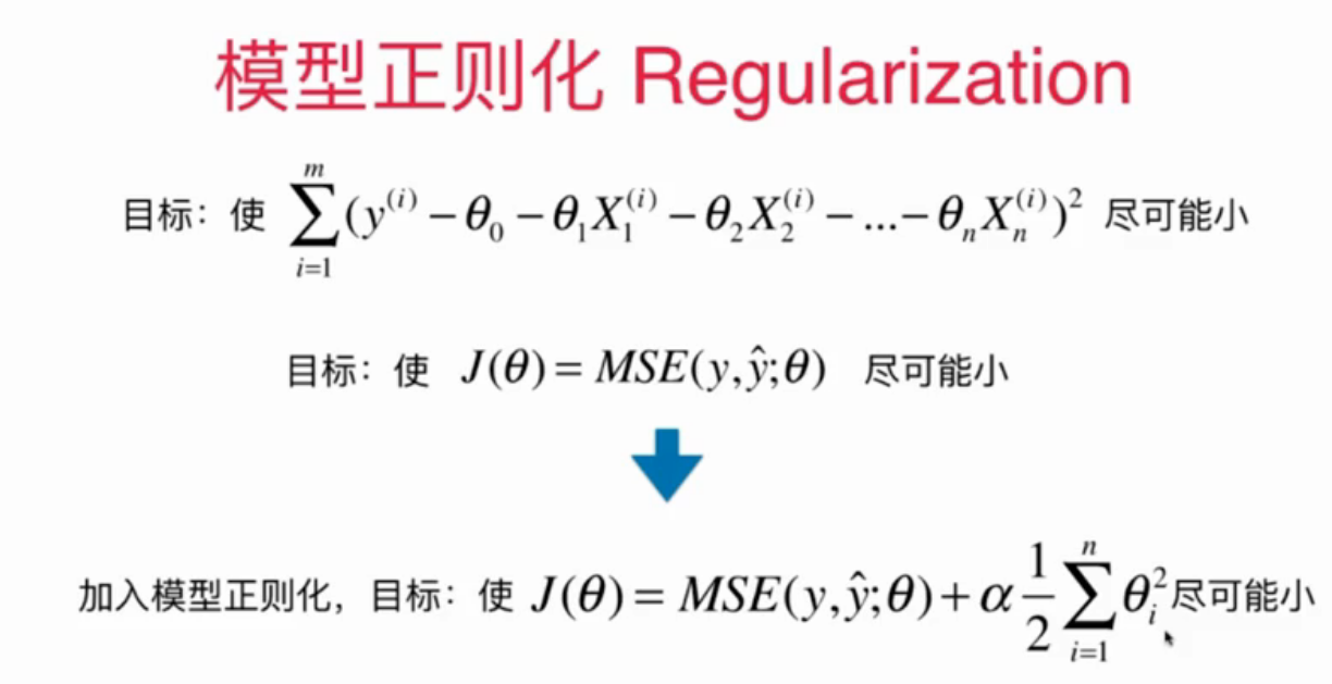

There are many ways to regularize models.

Ridge Regression

The problem of ridge regression is that the parameters in polynomial regression are too large. Here we add a sum of the square of the coefficients of the objective function to make the loss function as small as possible, so that the parameters can not be too large.

Polynomial regression is prone to over-fitting problems, that is, poor generalization ability on test data sets, ridge regression restricts the range of parameters, and can solve over-fitting problems to a certain extent. The following code is a comparison between the two:

import numpy as np 
from sklearn.preprocessing import PolynomialFeatures
from sklearn.preprocessing import StandardScaler
from sklearn.model_selection import train_test_split
from sklearn.pipeline import Pipeline
from sklearn.linear_model import LinearRegression
from sklearn.metrics import mean_squared_error
from sklearn.linear_model import Ridge

# Analog data set
np.random.seed(42)
x = np.random.uniform(-1.0,3.0,size=100)
X = x.reshape(-1,1)
y = 0.5 * x + 3 + np.random.normal(0,1,size=100)
np.random.seed(666)
X_train,X_test,y_train,y_test = train_test_split(X,y)

# Using Polynomial Regression
def PolynomialRegression(degree):
  return Pipeline([
    ('poly', PolynomialFeatures(degree=degree)),
    ('std_scaler', StandardScaler()),
    ('lin_reg', LinearRegression())
])

poly_reg = PolynomialRegression(degree=20)
poly_reg.fit(X_train,y_train)
y_poly_predict = poly_reg.predict(X_test)
mse = mean_squared_error(y_test,y_poly_predict)

print(mse)  # Output: 167.94061213110385


# Using Ridge Regression
def RidgeRegression(degree,alpha):
  return Pipeline([
    ('poly', PolynomialFeatures(degree=degree)),
    ('std_scaler', StandardScaler()),
    ('lin_reg', Ridge(alpha=alpha))
])

ridge_reg = RidgeRegression(20,0.01)
ridge_reg.fit(X_train,y_train)
y_ridge_predict = ridge_reg.predict(X_test)
mse2 = mean_squared_error(y_ridge_predict,y_test)
print(mse2)  # The output is: 1. 1959639082957925 and mse are better than Kedling regression.

LASSO Regression

Ridge regression is a method of model regularization, and LASSO is also a method of model regularization. The difference between them is the way to measure the overall size of theta. Ridge regression uses the square of theta, while LASSO uses the sum of absolute values of theta.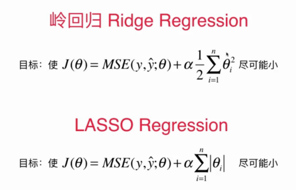

# Using LASSO regression
def LassoRegression(degree,alpha):
  return Pipeline([
    ('poly', PolynomialFeatures(degree=degree)),
    ('std_scaler', StandardScaler()),
    ('lin_reg', Lasso(alpha=alpha))
])

lasso_reg = LassoRegression(20,0.01)
lasso_reg.fit(X_train,y_train)
y_lasso_predict = lasso_reg.predict(X_test)
mse2 = mean_squared_error(y_lasso_predict,y_test)
print(mse2)  # Output: 1.1048334401791602

LASSO tends to make part of theta zero, so it is closer to a straight line than Ridge.
A feature with a parameter of 0 may be useless, so LASSO can be used for feature selection.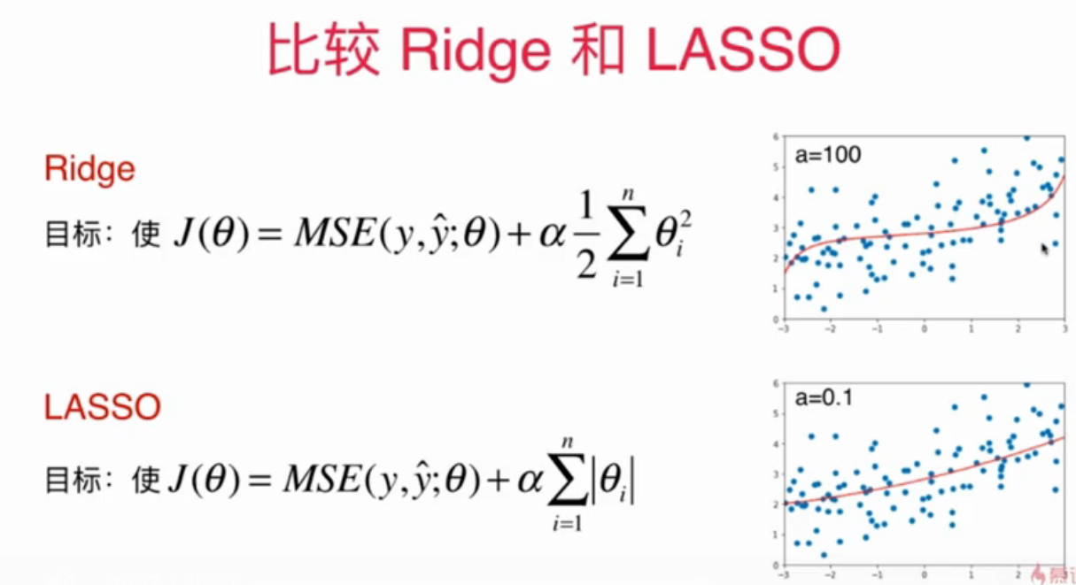

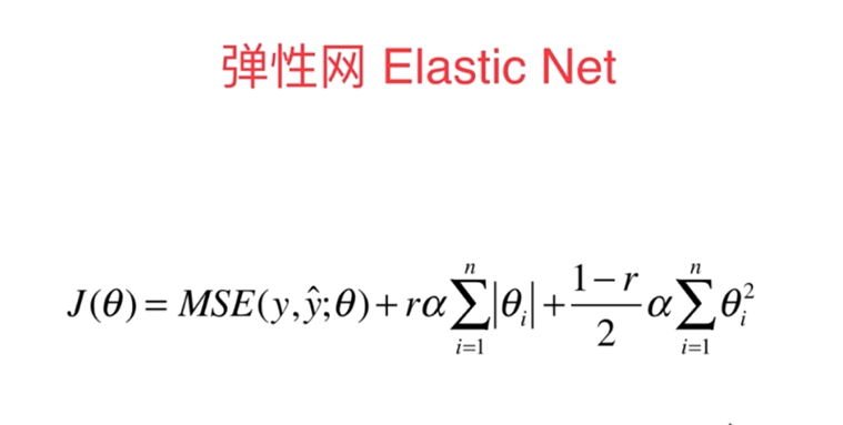
L1, L2 and Elastic Networks

Compare Ridge and LASSO again:
(Some concepts share the same idea)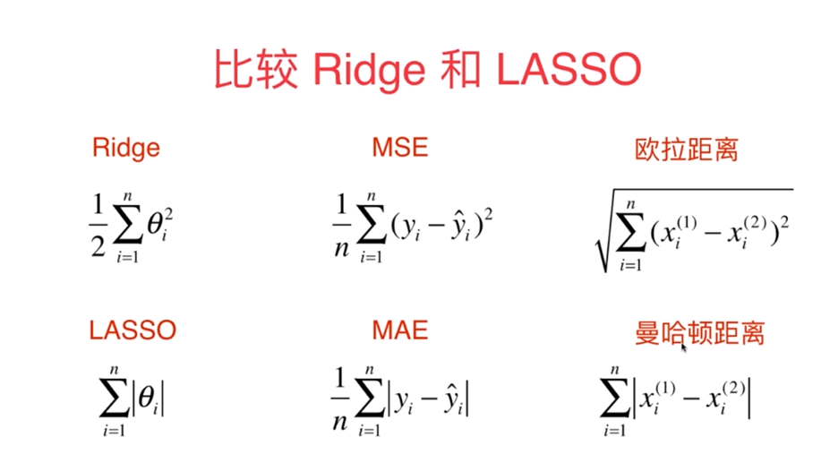



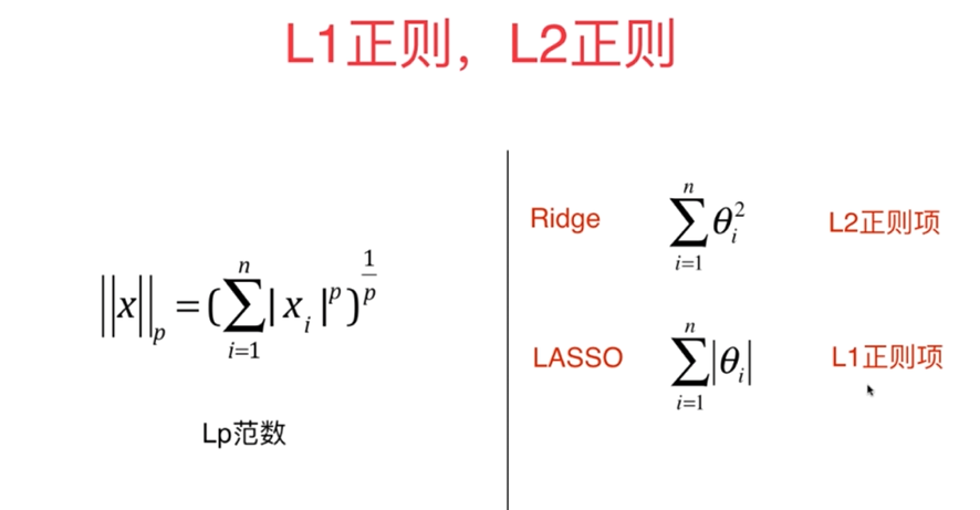
In practical application, ridge regression is usually used. The disadvantage of ridge regression is that it requires a large amount of calculation.
Elastic network combines the accurate characteristics of ridge regression and the characteristics of LASSO regression.