Brief background introduction

Today, the stupid younger martial brother exported a simulation data with comsol. Open it with matlab to see that it is a data length 189739 × 3 189739×3 one hundred and eighty-nine thousand seven hundred and thirty-nine × Matrix of 3

good heavens! Click in to see that the data format is OK. The first column is the x coordinate, the second column is the y coordinate, and the third column is the corresponding data value, but it is impossible to draw with ordinary drawing means. I asked younger martial brother, it turns out that the goods export the data values on the grid points in comsol, and his model uses triangular grid, so we can't use one M × N M×N M × N is represented by a matrix. Well, we can only use post-processing to draw the picture.

Try plot3

The plot3 function in matlab can map coordinates and values one by one, with the advantage of fast drawing speed. The disadvantage is the drawn point / line diagram. If you look closely, there will be gaps; A single plot3 command can only use one color, which is troublesome to change. Younger martial brother, this situation can only be drawn in the way of layered coloring

load('matlab.mat');
cc=colormap(hsv);%Coloring space

z_max = max(u_4(:,3));z_min = min(u_4(:,3));
z = u_4(:,3);
for i = 1:64
    u_ind = find(z_min+(z_max-z_min)*(i-1)/64<z & z<z_min+(z_max-z_min)*i/64);%Find the directory of data corresponding to the corresponding shading space
    plot3(u_4(u_ind,1),u_4(u_ind,2),u_4(u_ind,3),'.','Color',cc(i,:)); hold on;%Draw the corresponding color
end
view(0,90)

A dynamic diagram can be used to show this process:

The final result is as follows:

Does it look good? But when you zoom in, you can see:

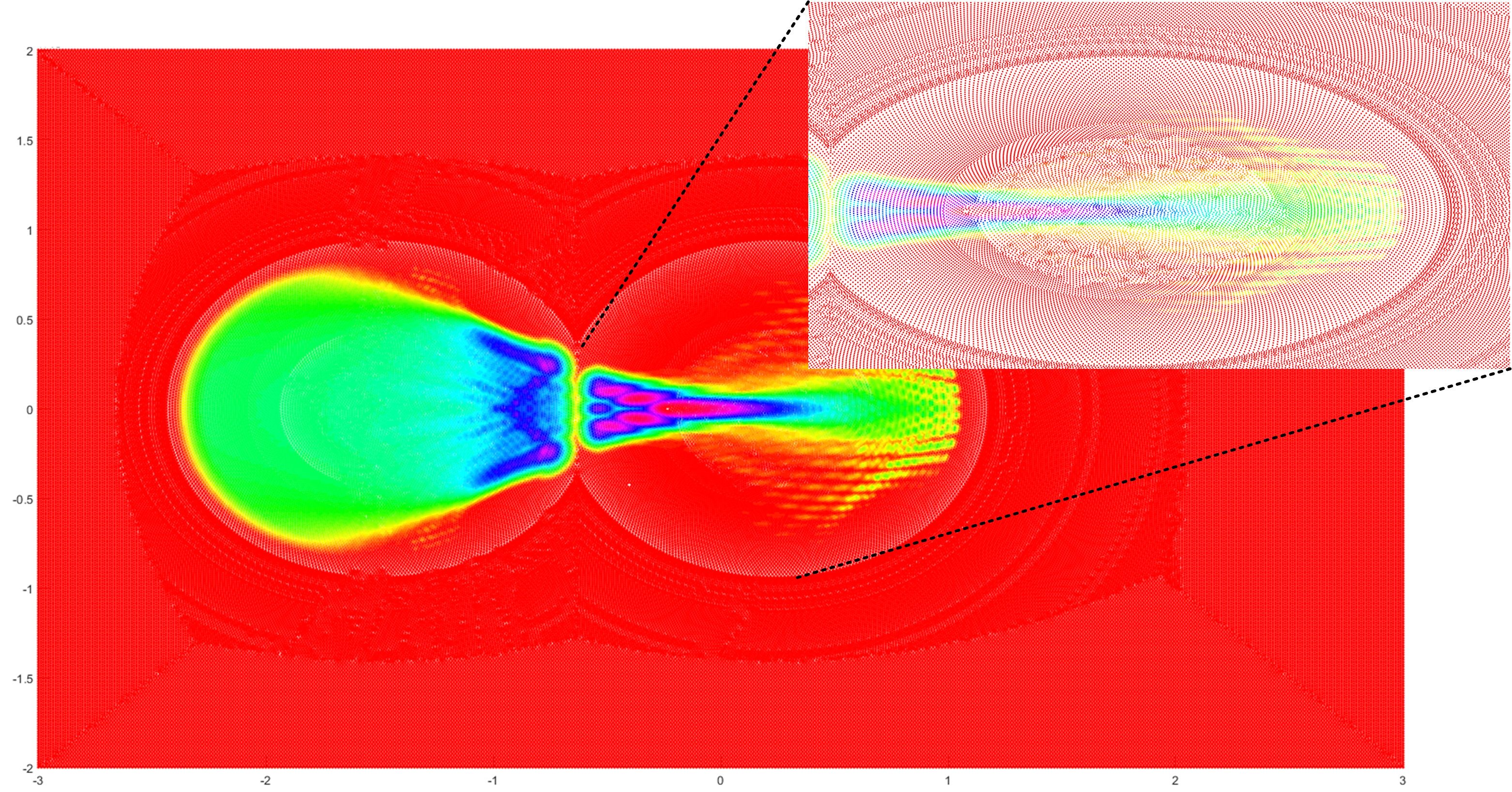
The grid points are not regular, but triangular. This greatly affects the subsequent processing process, and the data points are inconvenient to read and use, affecting the next data analysis.

Consider re extracting and integrating data points into a matrix

Construction matrix

Analyze the data before construction:

axis	minimum value	Maximum
X axis (m)	− 3 × 1 0 − 3 -3×10^{-3} −3×10−3	3 × 1 0 − 3 3×10^{-3} 3×10−3
Y axis (m)	− 2 × 1 0 − 3 -2×10^{-3} −2×10−3	2 × 1 0 − 3 2×10^{-3} 2×10−3
Z axis (data value)	41.4421	63.4641

I hope to put this data into one x n u m × y n u m x_{num}×y_{num} xnum​ × In the matrix of ynum ， for the convenience of debugging, use it first 127 × 127 127×127 one hundred and twenty-seven × 127, and then put the data into the matrix according to the coordinates. Since the amount of matrix data used is less than the total amount of data, it indicates that there are multiple data placed in the same matrix element, and the matrix elements need to be averaged. Therefore, the following small program is available:

clear all
close all
load('matlab.mat');
x_max = max(u_4(:,1));x_min = min(u_4(:,1));
y_max = max(u_4(:,2));y_min = min(u_4(:,2));
z_max = max(u_4(:,3));z_min = min(u_4(:,3));
x = u_4(:,1);
y = u_4(:,2);
z = u_4(:,3);
%% initialization
x_num = 128;
y_num = 128;
cx = linspace(x_min,x_max,x_num);
cy = linspace(y_min,y_max,y_num);
c_data = zeros(x_num-1,y_num-1);
for i = 1:x_num-1
    for j = 1:y_num-1
        u_find = find(cx(i)<x & x<cx(i+1) & cy(j)<y & y<cy(j+1));
        c_data(i,j) = mean(z(u_find));
    end
    disp(num2str(i))
end
figure;surf(c_data');view(0,90);shading interp;colormap(hsv)

The result is the following figure. It can be seen that the details of the figure are much less than those drawn by plot3, that is, the resolution is reduced, but this can be improved by changing the size of the storage matrix

But there is a fatal problem! The instant use time is too long!

Number of steps	Time (s)
125	4.8471
126	4.8808
127	4.9153

No way, this double cycle is bad. If it becomes 255 × 255 255×255 two hundred and fifty-five × 255 matrix, the time can reach 19.8258s

Traversal fill

No optimized version traversal filling

Considering that the double loop is actually the problem of addressing two-dimensional matrix elements and the low efficiency of find function, the problems to be solved are: 1. Improve the addressing efficiency, 2. Reduce or do not use find function.

The matrix address storage is arranged in order, but in the construction of the matrix, using the for loop will destroy the address order, resulting in longer addressing time, and the double loop will further prolong this time. Therefore, the total time consumption can be reduced by reducing the number of loop layers and retaining the address order. Secondly, the find function is actually a comparison function, which needs to traverse the data as a whole. One more find function is equivalent to one more loop. Therefore, the efficiency can be improved by not using or using less find function (such as using matrix operation to replace find function).

According to this idea, the way of traversing data and filling matrix can be used to improve the operation efficiency. Without saying a word, go to the code first

clear all
% close all
load('matlab.mat');
x_max = max(u_4(:,1));x_min = min(u_4(:,1));
y_max = max(u_4(:,2));y_min = min(u_4(:,2));
z_max = max(u_4(:,3));z_min = min(u_4(:,3));
x = u_4(:,1);
y = u_4(:,2);
z = u_4(:,3);
%%
x_num = 256;
y_num = 256;
x_delt = (x_max-x_min)/(x_num-1);
y_delt = (y_max-y_min)/(y_num-1);
cx = linspace(x_min,x_max,x_num-1);
cy = linspace(y_min,y_max,y_num-1);
c_data = zeros(x_num,y_num);
c_data_num = c_data;
c2 = nan * zeros(x_num,y_num);
x2 = floor((x-x_min)/x_delt)+1;
y2 = floor((y-y_min)/y_delt)+1;
tic
for i = 1:length(z)
   c_data(x2(i),y2(i)) = c_data(x2(i),y2(i))+z(i);
   c_data_num(x2(i),y2(i)) = c_data_num(x2(i),y2(i))+1;
%    if ~mod(i,10000) disp(num2str(i));end
end
toc
gx = c_data./c_data_num;
figure;surf(gx');view(0,90);shading interp;colormap(hsv)

In the above procedure, use c_data and c_data_num two matrices record the accumulated data and accumulation times respectively, and gx is the last generated matrix. The saved matrix size is 255 × 255 255×255 two hundred and fifty-five × 255, while the total running time is greatly reduced.

Time has passed 0.009621 Seconds.

The result is shown below. You can see that there are some uneven points at the boundary. There is no data at the boundary of the exported grid. If you have to level it, you can deal with it.

Optimized traversal filling

In fact, it has been optimized more than 2000 times, but in fact, there is still room for optimization. In the above non optimized version of traversal filling, a single loop is used to traverse the data, resulting in unnecessary addressing time consumption, which can be optimized through the matrix characteristics of matlab (in fact, it is a sentence, but the efficiency is greatly improved)

d_data = nan * c_data;
d_data((x2-1)*x_num+y2) = z; 

>>Time has passed 0.003155 Seconds.

The results are shown as follows:

Compared with before optimization, the difference is that when multiple data are placed in the same matrix element, one data is used instead of averaging the matrix elements. Therefore, the details will be slightly different. It is a pity

Unfortunately, it was solved, but the efficiency was reduced

tic
d_data((x2-1)*x_num+y2) = d_data((x2-1)*x_num+y2)+z; 
d_data_num((x2-1)*x_num+y2) = d_data_num((x2-1)*x_num+y2)+1; 
toc
>>Time has passed 0.008568 Seconds.