1 Basic Concepts

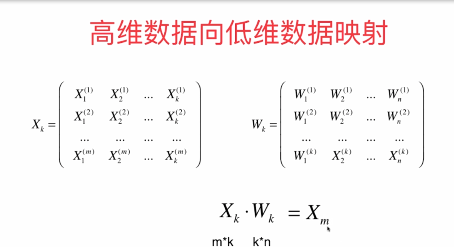
• PCA is principal component analysis. Principal component analysis, also known as principal component analysis, aims to use the idea of dimensionality reduction to transform multiple indicators into a few comprehensive indicators.
• In statistics, PCA is a technique to simplify data sets. It's a linear transformation. This transformation transforms the data into a new coordinate system, so that the first variance of any data projection is on the first coordinate (called the first principal component), the second variance is on the second coordinate (the second principal component), and so on.
• Principal component analysis (PCA) is often used to reduce the dimension of data sets, while maintaining the feature of the largest contribution of the opposite difference. This is achieved by retaining the low-order principal components and ignoring the high-order principal components. In this way, low-order components can often retain the most important aspects of the data. However, this is not certain. It depends on the specific application.

2 principle and mathematical derivation

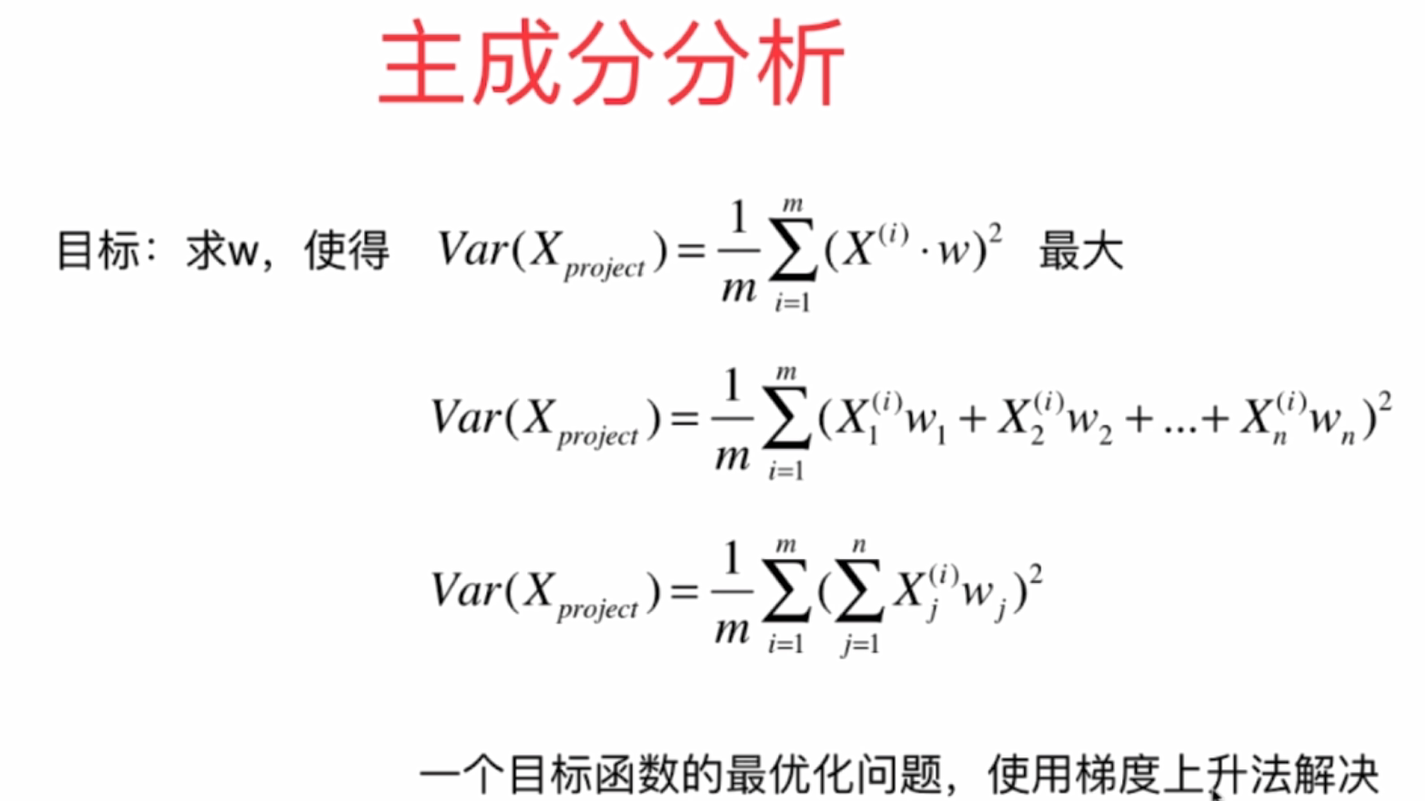
1. The gradient rise method is used in principal component analysis.
Characteristic
Principle: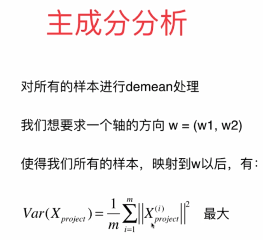

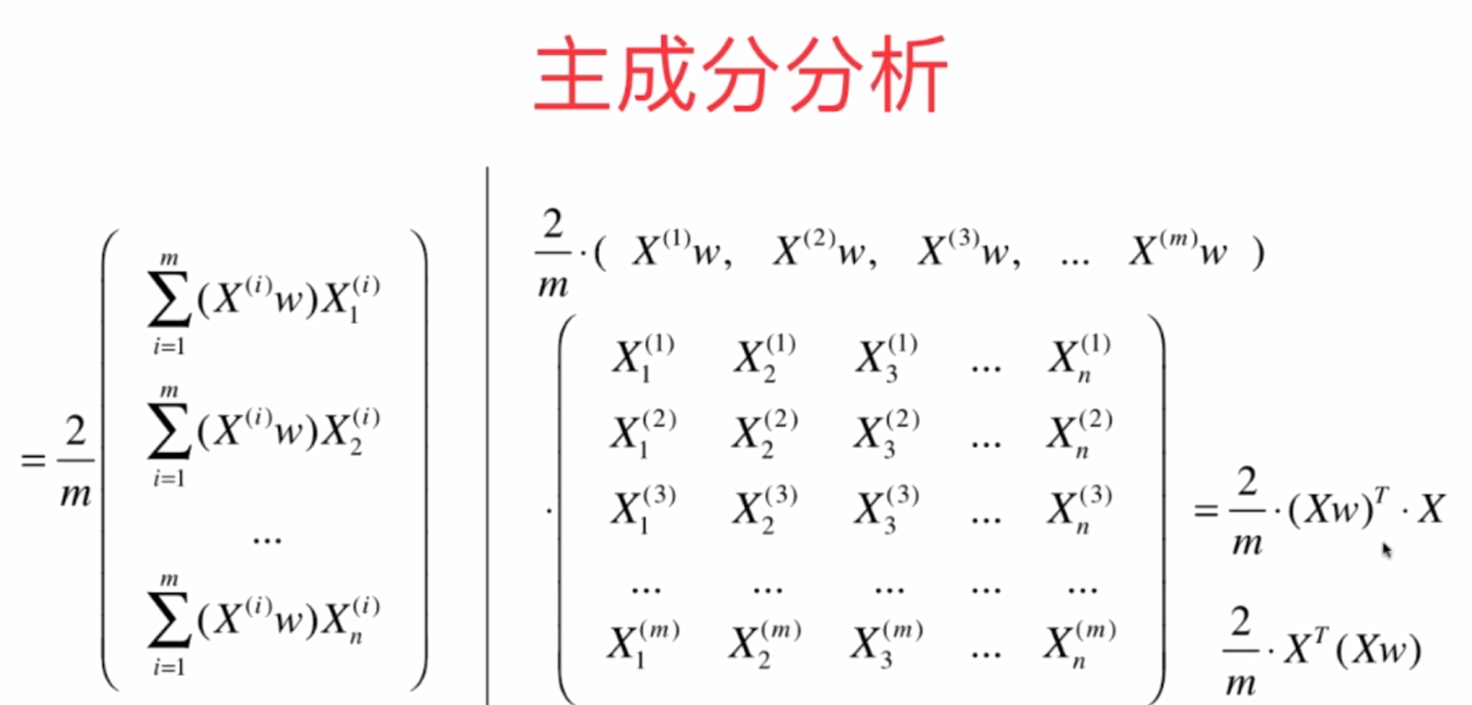
Mathematical derivation: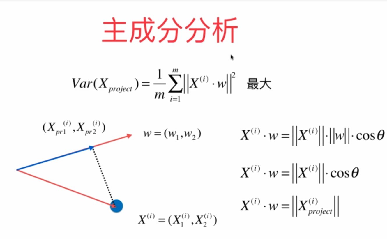

3 realize PCA algorithm by yourself

3.1 simulation of PCA by gradient rise method

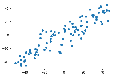
1. Simulation preparation of data

import numpy as np
import matplotlib.pyplot as plt
X = np.empty((100, 2))
X[:,0] = np.random.uniform(0., 100., size=100)
X[:,1] = 0.75 * X[:,0] + 3. + np.random.normal(0, 10., size=100)
plt.scatter(X[:,0], X[:,1])
plt.show()

2.demean operation (for each feature, set the mean value to 0 according to the column of X)

def demean(X):
    return X - np.mean(X, axis=0)
 
 X_demean = demean(X)

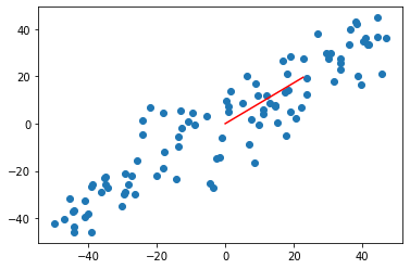
3. Use gradient rise method

def f(w, X):
    return np.sum((X.dot(w)**2)) / len(X)

def df_math(w, X):
    return X.T.dot(X.dot(w)) * 2. / len(X)

def df_debug(w, X, epsilon=0.0001):
    res = np.empty(len(w))
    for i in range(len(w)):
        w_1 = w.copy()
        w_1[i] += epsilon
        w_2 = w.copy()
        w_2[i] -= epsilon
        res[i] = (f(w_1, X) - f(w_2, X)) / (2 * epsilon)
    return res

def direction(w):
    return w / np.linalg.norm(w)  # Unit vectors

def gradient_ascent(df, X, initial_w, eta, n_iters = 1e4, epsilon=1e-8):
    
    w = direction(initial_w) 
    cur_iter = 0

    while cur_iter < n_iters:
        gradient = df(w, X)
        last_w = w
        w = w + eta * gradient
        w = direction(w) # Note 1: one unit direction at a time
        if(abs(f(w, X) - f(last_w, X)) < epsilon):
            break
            
        cur_iter += 1

    return w


initial_w =np.random.random(X.shape[1])  # Note that 2 cannot start with the 0 vector
w = gradient_ascent(df_math,X_demean,initial_w,eta)
plt.scatter(X_demean[:,0],X_demean[:,1])
plt.plot([0,w[0]*30],[0,w[1]*30],color = 'r')
plt.show()

Note 3: StandardScaler cannot be used to standardize data

4. The first principal component is calculated above. If other principal components are calculated, the first principal component should be subtracted and then put into it for solution.

#Other principal components
X2 = np.empty(X.shape)
for i in range(len(X)):
    X2[i] = X[i] - X[i].dot(w)*w    #Remove the first principal component
    
#Or it can be expressed as
X2 = X - X.dot(w).reshape(-1,1)*w

5. Find the first n principal components

def first_n_components(n,X,eta=0.01,n_iters=1e4,epsilon=1e-8):
    X_pca = X.copy()
    X_pca = demean(X_pca)
    res = []   # Main ingredients for storage
    for i in range(n):
        initial_w = np.random.random(X_pca.shape[1])
        w = first_component(df,X_pca,initial_w,eta)
        res.append(w)
        
        X_pca = X_pca - X_pca.dot(w).reshape(-1,1)*w
    return res

first_n_components(2,X)   #call

5. Realize PCA and encapsulate it

import numpy as np


class PCA:

    def __init__(self, n_components):
        """Initialization PCA"""
        assert n_components >= 1, "n_components must be valid"
        self.n_components = n_components
        self.components_ = None

    def fit(self, X, eta=0.01, n_iters=1e4):
        """Get data set X Before n Principal components"""
        assert self.n_components <= X.shape[1], \
            "n_components must not be greater than the feature number of X"

        def demean(X):
            return X - np.mean(X, axis=0)

        def f(w, X):
            return np.sum((X.dot(w) ** 2)) / len(X)

        def df(w, X):
            return X.T.dot(X.dot(w)) * 2. / len(X)

        def direction(w):
            return w / np.linalg.norm(w)

        def first_component(X, initial_w, eta=0.01, n_iters=1e4, epsilon=1e-8):

            w = direction(initial_w)
            cur_iter = 0

            while cur_iter < n_iters:
                gradient = df(w, X)
                last_w = w
                w = w + eta * gradient
                w = direction(w)
                if (abs(f(w, X) - f(last_w, X)) < epsilon):
                    break

                cur_iter += 1

            return w

        X_pca = demean(X)
        self.components_ = np.empty(shape=(self.n_components, X.shape[1]))
        for i in range(self.n_components):
            initial_w = np.random.random(X_pca.shape[1])
            w = first_component(X_pca, initial_w, eta, n_iters)
            self.components_[i,:] = w

            X_pca = X_pca - X_pca.dot(w).reshape(-1, 1) * w

        return self

    def transform(self, X):
        """Given X，Mapping to principal components"""
        assert X.shape[1] == self.components_.shape[1]

        return X.dot(self.components_.T)

    def inverse_transform(self, X):
        """Given X，Reverse mapping back to the original feature space"""
        assert X.shape[1] == self.components_.shape[0]

        return X.dot(self.components_)

    def __repr__(self):
        return "PCA(n_components=%d)" % self.n_components

1. Dimension reduction of data
   
   

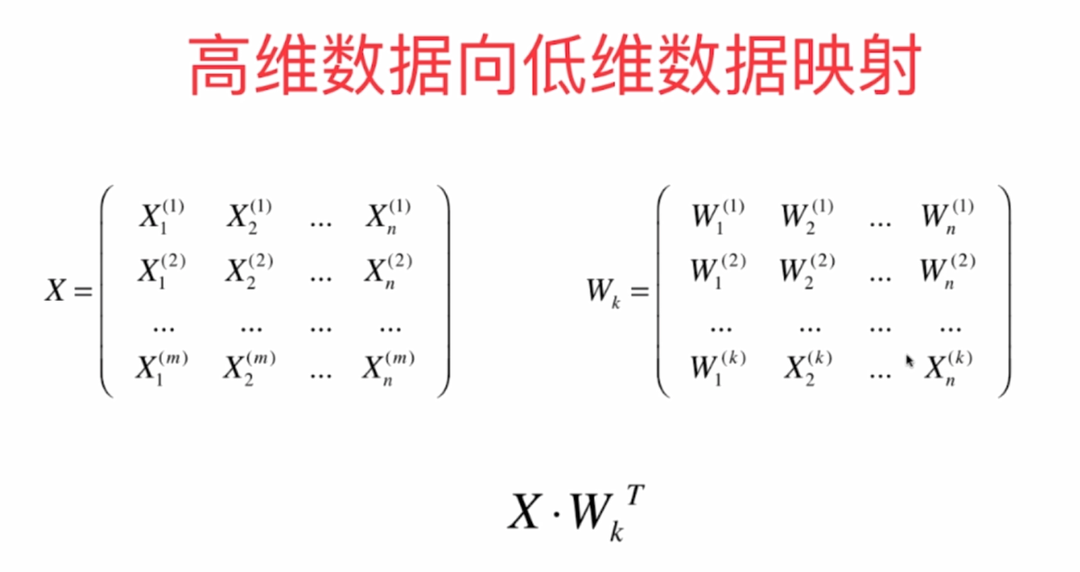
import numpy as np
import matplotlib.pyplot as plt
X = np.empty((100, 2))
X[:,0] = np.random.uniform(0., 100., size=100)
X[:,1] = 0.75 * X[:,0] + 3. + np.random.normal(0, 10., size=100)
from playML.PCA import PCA

pca = PCA(n_components=2)
pca.fit(X)
pca.components_
pca = PCA(n_components=1)
pca.fit(X)
X_reduction = pca.transform(X)
X_reduction.shape
X_restore = pca.inverse_transform(X_reduction)
X_restore.shape
plt.scatter(X[:,0], X[:,1], color='b', alpha=0.5)
plt.scatter(X_restore[:,0], X_restore[:,1], color='r', alpha=0.5)
plt.show()

N? Components represents the required principal components. X ﹣ reduction is the matrix after dimension reduction. X ﹣ restore represents the matrix recovered after dimension reduction.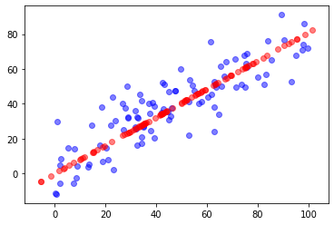

PCA algorithm in 4 sklearn

1. Reduce dimension by pca

from sklearn.decomposition import PCA
pca = PCA(n_components=1)
pca.fit(X)
pca.components_
X_reduction = pca.transform(X)
X_restore = pca.inverse_transform(X_reduction)

2. After dimension reduction by PCA with specific handwritten digit recognition, KNN is used for classification

import numpy as np
import matplotlib.pyplot as plt
from sklearn import datasets
digits = datasets.load_digits()
X = digits.data
y = digits.target
from sklearn.model_selection import train_test_split

X_train, X_test, y_train, y_test = train_test_split(X, y, random_state=666)

from sklearn.decomposition import PCA

pca = PCA(n_components=2)
pca.fit(X_train)
X_train_reduction = pca.transform(X_train)
X_test_reduction = pca.transform(X_test)

knn_clf = KNeighborsClassifier()
knn_clf.fit(X_train_reduction, y_train)
knn_clf.score(X_test_reduction, y_test)

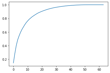
3. Take the number of principal component components to explain the principal component fraction (PCA. Explained "variance" explained by principal component)

from sklearn.decomposition import PCA

pca = PCA(n_components=X_train.shape[1])
pca.fit(X_train)

plt.plot([i for i in range(X_train.shape[1])], 
         [np.sum(pca.explained_variance_ratio_[:i+1]) for i in range(X_train.shape[1])])
plt.show()

Or use the following:

pca = PCA(0.95)
pca.fit(X_train)
pca.n_components_
X_train_reduction = pca.transform(X_train)
X_test_reduction = pca.transform(X_test)

knn_clf = KNeighborsClassifier()
knn_clf.fit(X_train_reduction, y_train)
knn_clf.score(X_test_reduction, y_test)

PCA. N ﹣ components ﹣ is the number of all principal components whose corresponding proportion is 0.95
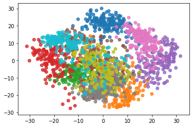
4. Data visualization after dimensionality reduction

%%time 
pca = PCA(n_components=2)
pca.fit(X)
X_reduction = pca.transform(X)
for i in range(10):
    plt.scatter(X_reduction[y==i,0], X_reduction[y==i,1], alpha=0.8)

5 other applications of PCA

1. Noise reduction by PCA

from sklearn import datasets

digits = datasets.load_digits()
X = digits.data
y = digits.target
noisy_digits = X + np.random.normal(0, 4, size=X.shape)
example_digits = noisy_digits[y==0,:][:10]
for num in range(1,10):
    example_digits = np.vstack([example_digits, noisy_digits[y==num,:][:10]])
example_digits.shape
def plot_digits(data):
    fig, axes = plt.subplots(10, 10, figsize=(10, 10),
                             subplot_kw={'xticks':[], 'yticks':[]},
    gridspec_kw=dict(hspace=0.1, wspace=0.1)) 
    for i, ax in enumerate(axes.flat):
        ax.imshow(data[i].reshape(8, 8),
                  cmap='binary', interpolation='nearest',
                  clim=(0, 16))

    plt.show()
    
plot_digits(example_digits)
pca = PCA(0.5).fit(noisy_digits)
pca.n_components_
components = pca.transform(example_digits)
filtered_digits = pca.inverse_transform(components)
plot_digits(filtered_digits)
components = pca.transform(example_digits)
filtered_digits = pca.inverse_transform(components)
plot_digits(filtered_digits)

Using the positive and negative transformation of PCA to remove the existing noise
2. feature faces

import numpy as np
import matplotlib.pyplot as plt
from sklearn.datasets import fetch_lfw_people
faces = fetch_lfw_people()
faces.keys()
faces.data.shape
faces.target_names
faces.images.shape
random_indexes = np.random.permutation(len(faces.data))
X = faces.data[random_indexes]
example_faces = X[:36,:]
example_faces.shape
def plot_faces(faces):
    
    fig, axes = plt.subplots(6, 6, figsize=(10, 10),
                         subplot_kw={'xticks':[], 'yticks':[]},
    gridspec_kw=dict(hspace=0.1, wspace=0.1)) 
    for i, ax in enumerate(axes.flat):
        ax.imshow(faces[i].reshape(62, 47), cmap='bone')
    plt.show()
    
plot_faces(example_faces)

#  Characteristic faces
from sklearn.decomposition import PCA 
pca = PCA(svd_solver='randomized')
pca.fit(X)
pca.components_.shape
plot_faces(pca.components_[:36,:])


faces2 = fetch_lfw_people(min_faces_per_person=60)
faces2.data.shape
faces2.target_names
len(faces2.target_names)
len(faces2.target_names)

5 Summary

1. When PCA is used for dimensionality reduction, it is suitable for data with more features. However, it should be noted that the data cannot be standardized, otherwise the PCA dimension reduction will fail. The basic principle is to use the gradient rise method to maximize the variance. Standardization will change the variance, so it cannot be standardized.
2. PCA can also be used for noise reduction. In the process of dimension reduction, the main components are actually extracted and the noise is filtered indirectly, so the accuracy of the model can be improved.
3. pca can also be used to represent feature faces.