1. tsp issues

The TSP problem is the traveler problem. The classic TSP can be described as: a merchandise salesman wants to go to several cities to sell his goods. The salesman starts from one city and needs to go through all the cities before he returns to his starting place.How to choose a course to minimize the overall trip.From a graph theory point of view, the problem is essentially to find a Hamilton circuit with the smallest weight in a weighted undirected graph.

There are many different ways to ask a traveler's question. Recently, I have done several questions about TSP, which are summarized below.Since most TSP problems are NP-Hard, it is difficult to get any efficient polynomial-level algorithms. The general algorithms used tend to be violent search and pressure DP, where pressure DP is used to solve them.The number of locations given by most TSP problems is very small.

Considering the classical TSP problem, it is not difficult to get the state transfer equation if using pressure DP to compress each site visit as binary 1/0:
dp[S][i] = min(dp[S][i], dp[S ^ (1 << (i - 1))][k] + dist[k][i])
S stands for the current state, i (from 1) indicates that the last place visited when the current state is reached is the ith place
k is all the places in S that are visited that are different from i.
dist represents the shortest path between two points.
And initialization:
DP[S][i] = dist[start][i](S == 1<<(i - 1))
If you are unfamiliar with pressure dp for the first time, think carefully about the meaning of the above formula, which is the key to most TSP problems.

2. nsga-II algorithm

1 NSGA algorithm

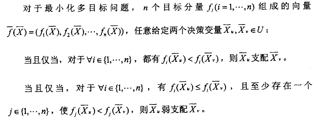
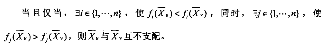
1.1 Paerot Dominance

1.2 Pareto Optimal Solution Definition

Multi-objective optimization problems differ greatly from single-objective optimization problems.When there is only one objective function, people seek the best solution, which is superior to all other solutions, usually the global maximum or minimum, that is, the global optimal solution.When there are multiple objectives, it is difficult to find a solution to make all the objective functions optimal at the same time because there are conflicts among them. That is, one solution may be the best for one objective function, but not the best or even the worst for other objective functions.Therefore, for multi-objective optimization problems, there usually exists a set of solutions, which cannot be compared with each other in terms of all objective functions. It is characterized by the inability to improve any objective function without weakening at least one other objective function.This solution is called a nondominated solution or Pareto optimal solution Soluitons), defined as follows:

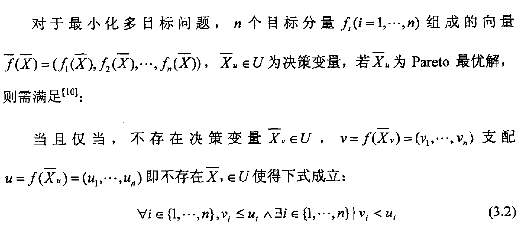
That is, there is no other value to dominate Xu.

2. General NSGA process

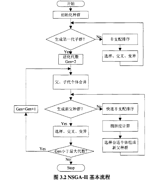
The non-dominant hierarchical approach adopted by NSGA allows better individuals greater chance of inheriting to the next generation.The fitness sharing strategy enables individuals on the quasi-Pareto surface to be evenly distributed, maintains population diversity, overcomes overbreeding of superindividuals, and prevents premature convergence.The flowchart is as follows:

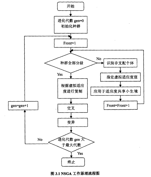
The main difference between NSGA and simple genetic algorithm is that the algorithm layers according to the dominance relationship between individuals before the selection operator is executed.The selection operator, crossover operator and mutation operator are not different from simple genetic algorithm.

As you can see from the graph, the algorithm first determines if the population is fully graded, then on the basis of the grading, it adjusts the virtual fitness value using the niche technology based on crowding strategy, determines the virtual fitness value of each population, and then according to the size of the virtual fitness value,Identify a population (genetic algorithm) to prioritize for processing.

2.1 Non-dominant Sorting

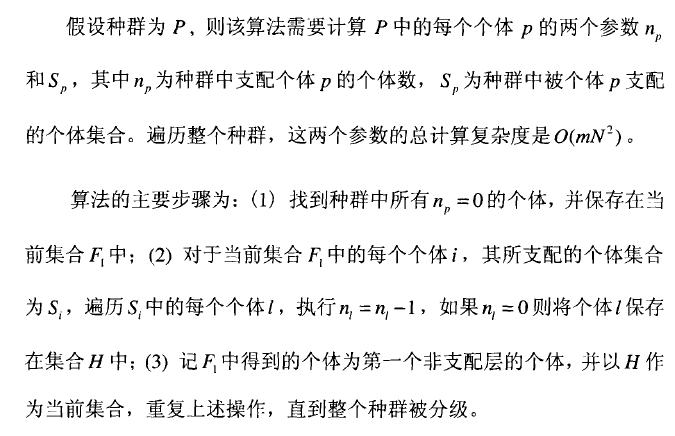
Considering a population with K (K>1) as the number of objective functions and N as the size of the population, the non-dominant sorting algorithm can be used to stratify the population by following steps:

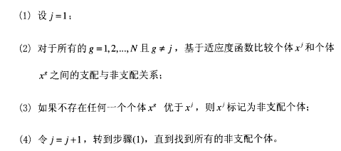
The set of non-dominant individuals derived from the above steps is the first level of non-dominant layer of the population.Next, ignore the marked non-dominant individuals and follow step (1) 1 (4) to obtain the second level of non-dominance.And so on until the entire population is classified.

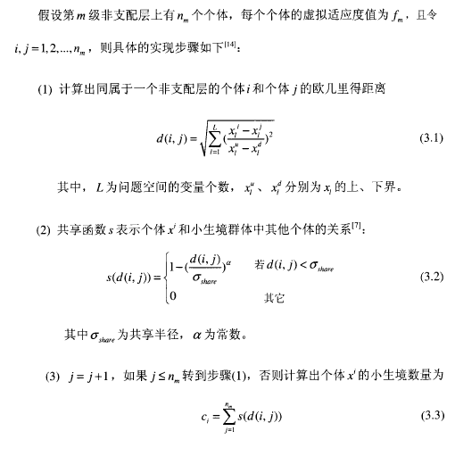
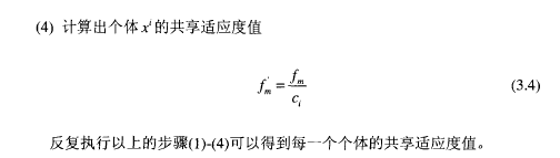
2.2 Determination of virtual fitness value

In the process of non-dominant population sorting, a virtual fitness value is assigned to each non-dominant layer.The larger the series, the smaller the virtual fitness value.Conversely, the higher the virtual fitness value is.This ensures that the lower-ranking non-dominant individuals have more chance to be selected for the next generation in the selection operation, making the algorithm converge to the optimal region at the fastest speed.On the other hand, in order to obtain a well-distributed Areto optimal solution set, the diversity of individuals at the current non-dominant layer is guaranteed.NSGA introduces the technology of niche based on crowding strategy (NIChe), that is, the fitness sharing function is used to re-specify the virtual fitness values that were originally specified.

3. NSGAII algorithm

The basic idea of NSGA-II algorithm is: first, the initial population of N is randomly generated, and then the first generation of the descendant population is obtained by genetic algorithm selection, crossover and mutation after non-dominant sorting.Secondly, starting from the second generation, the parent population and the offspring population are merged, fast non-dominant sorting is performed, and the crowding degree of the individual in each non-dominant layer is calculated, and the appropriate individual is selected to form a new parent population according to the non-dominant relationship and the crowding degree of the individual.Finally, a new descendant population is generated from the basic operations of the genetic algorithm: and so on, until the condition for the end of the program is met.The corresponding program flowchart is shown in the following figure.

3.1 Fast Non-dominant Sorting Algorithm

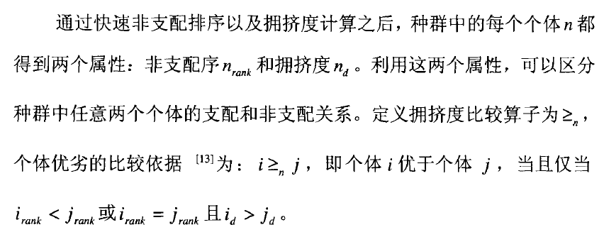
3.2 Comparing Operator of Congestion and Congestion

Crowding is the density of the surrounding individuals of a given individual in a population, which can be visually represented as an individual.There are only individuals around.The rectangle of its largest rectangle, denoted by nd,

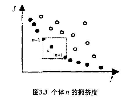
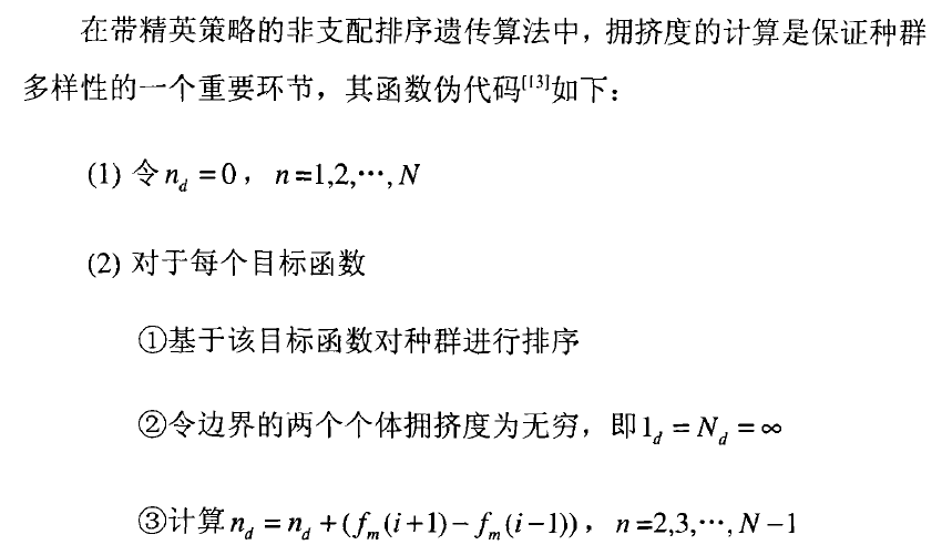
The algorithm for congestion is as follows:

3.3 Congestion Comparing Operator

3. Partial Codes

% function NSGA_2
clc;clear;
tic;
%% Initialization
PopSize=200;%Population size 
MaxIteration =300;%Maximum number of iterations
R=50;
% location1=load('location1_100.txt');%Optimize 100 cities
% location2=load('A_location2_100.txt');
location1=load('location1.txt');
location2=load('location2.txt');
CityNum =size(location1,2);%Number of cities
V=CityNum;
M=2;
pc=0.8;pm=0.9;
for i=1:PopSize
    chromosome(i,1:CityNum)=randperm(CityNum);
    chromosome(i,CityNum+1:CityNum+2)=costfunction(chromosome(i,1:CityNum),location1,location2);
end
chromosome= non_domination_sort_mod(chromosome);%Make the last column of decomposition the last column of congestion and the second column the number of rankings
index=find(chromosome(:,103)==1);
costrep=chromosome(index,101:102);%The first level is the non-inferior solution

%% Main cycle
pool = round(PopSize/2);  %Mutation pool size

for Iteration=1:MaxIteration
    if ~mod(Iteration,10)
        fprintf('current iter:%d\n',Iteration)
        disp([' Number of Repository Particles = ' num2str(size(costrep,1))]);

            scro(2,m1)=tt;
        end
        scro_cost(1,:)=costfunction(scro(1,:),location1,location2);
        scro_cost(2,:)=costfunction(scro(2,:),location1,location2);
        offspring_var=[offspring_var;scro];%solution
        offspring_cost=[offspring_cost;scro_cost];%Fitness
        
    end
    offspring_chromosome(:,1:V)=offspring_var;
    offspring_chromosome(:,V+1:V+M)=offspring_cost;
    
    main_pop = size(chromosome,1);
    offspring_pop = size(offspring_chromosome,1);
    intermediate_chromosome(1:main_pop,:) = chromosome;
    intermediate_chromosome(main_pop + 1 :main_pop + offspring_pop,1 : M+V) = ...
        offspring_chromosome;
    intermediate_chromosome = ...
        non_domination_sort_mod(intermediate_chromosome);
    %% Choice
    
    chromosome = replace_chromosome(intermediate_chromosome,PopSize);
    
    
    index=find(intermediate_chromosome(:,103)==1);
    costrep=intermediate_chromosome(index,101:102);
    cost=intermediate_chromosome(:,101:102);
        if ~mod(Iteration,1)
    
            figure (1)
            plot(costrep(:,1),costrep(:,2),'r*',cost(:,1),cost(:,2),'kx');
            xlabel('F1');ylabel('F2');
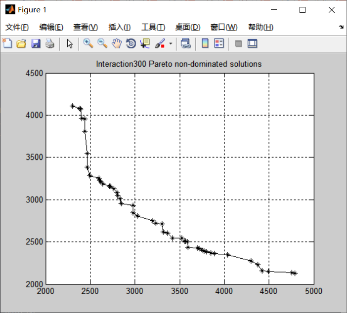
            title(strcat('Interaction ',num2str(Iteration), ' Pareto non-dominated solutions'));
            %          hold on
        end
    if ~mod(Iteration,MaxIteration)
        %             if ~mod(Iteration,1)
        fun_pf=costrep;
        [fun_pf,~]=sortrows(fun_pf,1);
        plot(fun_pf(:,1),fun_pf(:,2),'k*-');
        title(strcat('Interaction ',num2str(Iteration), ' Pareto non-dominated solutions'));
        hold on;
        grid on;
    end
end

4. Simulation results

 

5. References

[1] Liu Shengjun, Geng Sheng Tong, Xie Fei. Application of New Oriented Crossing in NSGA-II Solving Multi-objective TSP Problem [J]. Electronic Technology and Software Engineering, 2017 (06): 154.