Over fitting, under fitting

1. Training error and generalization error
   Training error refers to the error of the model in the training data set;
   Test error refers to the expected error of the model on any test data sample, and is often approximated by the error on the test data set.
2. Model selection
   In the training process, in order to get better parameters, we need a validation data set. This is usually obtained from the partition of training data sets. K-fold cross validation is usually used in partition. Generally speaking, K=10. The final results are all averaged.
3. Over fitting, under fitting
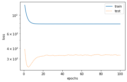
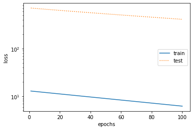
   From the performance of training error and generalization error, the model can not get lower training error, we call this phenomenon underfitting; the training error of the model is far less than its error in the test data set, we call this phenomenon over fitting. These two phenomena are usually related to the complexity of the model and the size of the training data set.

Polynomial function fitting experiment

When the model is n-order polynomial (the more N, the higher the model complexity), given the training data set, the relationship between the model complexity and the error is shown in the following figure:

It is worth mentioning here that in general, in DL, the training data set is always insufficient while the model is strong enough, so there will be more cases of over fitting.

%matplotlib inline
import torch
import numpy as np
import sys
sys.path.append("/home/kesci/input")
import d2lzh1981 as d2l
print(torch.__version__)

#Initialize model parameters
n_train, n_test, true_w, true_b = 100, 100, [1.2, -3.4, 5.6], 5
features = torch.randn((n_train + n_test, 1))
poly_features = torch.cat((features, torch.pow(features, 2), torch.pow(features, 3)), 1) 
labels = (true_w[0] * poly_features[:, 0] + true_w[1] * poly_features[:, 1]
          + true_w[2] * poly_features[:, 2] + true_b)
labels += torch.tensor(np.random.normal(0, 0.01, size=labels.size()), dtype=torch.float)

#Definition model
def semilogy(x_vals, y_vals, x_label, y_label, x2_vals=None, y2_vals=None,
             legend=None, figsize=(3.5, 2.5)):
    # d2l.set_figsize(figsize)
    d2l.plt.xlabel(x_label)
    d2l.plt.ylabel(y_label)
    d2l.plt.semilogy(x_vals, y_vals)
    if x2_vals and y2_vals:
        d2l.plt.semilogy(x2_vals, y2_vals, linestyle=':')
        d2l.plt.legend(legend)

num_epochs, loss = 100, torch.nn.MSELoss()

def fit_and_plot(train_features, test_features, train_labels, test_labels):
    # Initialize network model
    net = torch.nn.Linear(train_features.shape[-1], 1)
    # According to the Linear document, pytorch has initialized the parameters, so we won't initialize them manually here
    
    # Set batch size
    batch_size = min(10, train_labels.shape[0])    
    dataset = torch.utils.data.TensorDataset(train_features, train_labels)      # Set up datasets
    train_iter = torch.utils.data.DataLoader(dataset, batch_size, shuffle=True) # Set how to get data
    
    optimizer = torch.optim.SGD(net.parameters(), lr=0.01)                      # Set the optimization function and use the random gradient descent optimization
    train_ls, test_ls = [], []
    for _ in range(num_epochs):
        for X, y in train_iter:                                                 # Take a batch of data
            l = loss(net(X), y.view(-1, 1))                                     # Input to the network to calculate the output, and compare with the label to obtain the loss function
            optimizer.zero_grad()                                               # Optimization of gradient clearing to prevent interference of gradient accumulation
            l.backward()                                                        # Seeking gradient
            optimizer.step()                                                    # Iterative optimization function for parameter optimization
        train_labels = train_labels.view(-1, 1)
        test_labels = test_labels.view(-1, 1)
        train_ls.append(loss(net(train_features), train_labels).item())         # Save training loss to train? LS
        test_ls.append(loss(net(test_features), test_labels).item())            # Save the test loss to test? LS
    print('final epoch: train loss', train_ls[-1], 'test loss', test_ls[-1])    
    semilogy(range(1, num_epochs + 1), train_ls, 'epochs', 'loss',
             range(1, num_epochs + 1), test_ls, ['train', 'test'])
    print('weight:', net.weight.data,
          '\nbias:', net.bias.data)

#test
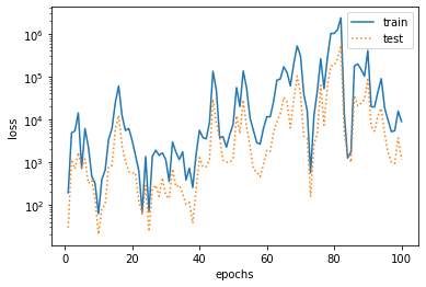
fit_and_plot(poly_features[:n_train, :], poly_features[n_train:, :], labels[:n_train], labels[n_train:]) #normal
fit_and_plot(features[:n_train, :], features[n_train:, :], labels[:n_train], labels[n_train:]) #Under fitting
fit_and_plot(poly_features[0:2, :], poly_features[n_train:, :], labels[0:2], labels[n_train:]) #Over fitting

• Third order polynomial fitting (normal)
  

Although the model here is a linear model, the input sample characteristics are polynomial calculated, so the linear combination with parameters is a polynomial model.

• Linear fit (under fit)
  
• Too few training sets (over fitting)
  

Methods to prevent over fitting

1. L2 regularization (also called weight attenuation)
   By adding L2 regularization, we can prevent the extreme large of individual parameters, so as to prevent over fitting. Under the global minimum constraint, add L2 regularization term to the loss function:
   ℓ(w1,w2,b)+λ2n∣w∣2 \ell\left(w_{1}, w_{2}, b\right)+\frac{\lambda}{2 n}|w|^{2} ℓ(w1​,w2​,b)+2nλ​∣w∣2

optimizer_w = torch.optim.SGD(params=[net.weight], lr=lr, weight_decay=wd) # Attenuation of weight parameters

1. dropout (also called drop out method)
   Discarding method can inactivate some units (i.e. set the corresponding value to 0) with a certain probability to avoid over dependence on some neurons in the training process. The following formula proves that the discard method does not change the input expectation.
   hi′=ξi1−phiE(hi′)=E(ξi)1−phi=hi h_{i}^{\prime}=\frac{\xi_{i}}{1-p} h_{i} \\ E\left(h_{i}^{\prime}\right)=\frac{E\left(\xi_{i}\right)}{1-p} h_{i}=h_{i} hi′​=1−pξi​​hi​E(hi′​)=1−pE(ξi​)​hi​=hi​

def dropout(X, drop_prob):
    X = X.float()
    assert 0 <= drop_prob <= 1
    keep_prob = 1 - drop_prob
    # In this case, all elements are discarded
    if keep_prob == 0:
        return torch.zeros_like(X)
    mask = (torch.rand(X.shape) < keep_prob).float()
    print(mask)
    
    return mask * X / keep_prob
# Instructions
def net(X, is_training=True):
    X = X.view(-1, num_inputs)
    H1 = (torch.matmul(X, W1) + b1).relu()
    if is_training:  # Use discard only when training models
        H1 = dropout(H1, drop_prob1)  # Add a discard layer after the first layer is fully connected
    H2 = (torch.matmul(H1, W2) + b2).relu()
    if is_training:
        H2 = dropout(H2, drop_prob2)  # Add drop layer after full connection of the second layer
    return torch.matmul(H2, W3) + b3

#pytorch implementation
nn.Dropout(drop_prob1)

Some words

Some questions:

1. How to see it is over fitting? What are the ways to prevent over fitting?
2. What are the principles of L2 regularization and dropout to prevent over fitting? How do I implement them with pytorch?