Grayscale Grayscale
import cv2 #opencv reads in BGR format

img=cv2.imread('cat.jpg')
img_gray = cv2.cvtColor(img,cv2.COLOR_BGR2GRAY)
img_gray.shape

cv2.imshow("img_gray", img_gray)
cv2.waitKey(0)
cv2.destroyAllWindows()
HSV
H - Tone (main wavelength).
S-Saturation (shadows of purity/color).
V value (intensity)
cv2.imshow("hsv", hsv)
cv2.waitKey(0)
cv2.destroyAllWindows()
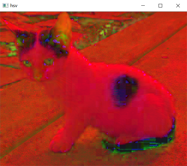
Image Threshold
ret, dst = cv2.threshold(src, thresh, maxval, type)
-
src: Input graph, which can only input a single channel image, usually a grayscale image
-
dst: output graph - thresh: threshold
-
maxval: The value assigned when the pixel value exceeds (or is smaller than) the threshold, determined by type
-
Type: The type of binarization operation that contains the following five types:
cv2.THRESH_BINARY; cv2.THRESH_BINARY_INV; cv2.THRESH_TRUNC;
cv2.THRESH_TOZERO;cv2.THRESH_TOZERO_INV-
cv2.THRESH_BINARY over threshold take maxval (maximum), otherwise 0
-
Reverse of cv2.THRESH_BINARY_INV THRESH_BINARY
-
The greater than threshold part of cv2.THRESH_TRUNC is set as the threshold value, otherwise the unchanged cv2.THRESH_TOZERO greater than the threshold part is not changed, otherwise set to 0
-
Reverse of cv2.THRESH_TOZERO_INV THRESH_TOZERO
-
ret, thresh1 = cv2.threshold(img_gray, 127, 255, cv2.THRESH_BINARY)
ret, thresh2 = cv2.threshold(img_gray, 127, 255, cv2.THRESH_BINARY_INV)
ret, thresh3 = cv2.threshold(img_gray, 127, 255, cv2.THRESH_TRUNC)
ret, thresh4 = cv2.threshold(img_gray, 127, 255, cv2.THRESH_TOZERO)
ret, thresh5 = cv2.threshold(img_gray, 127, 255, cv2.THRESH_TOZERO_INV)

titles = ['Original Image', 'BINARY', 'BINARY_INV', 'TRUNC', 'TOZERO', 'TOZERO_INV']
images = [img, thresh1, thresh2, thresh3, thresh4, thresh5]

for i in range(6):
    plt.subplot(2, 3, i + 1), plt.imshow(images[i], 'gray')
    plt.title(titles[i])
    plt.xticks([]), plt.yticks([])
plt.show()
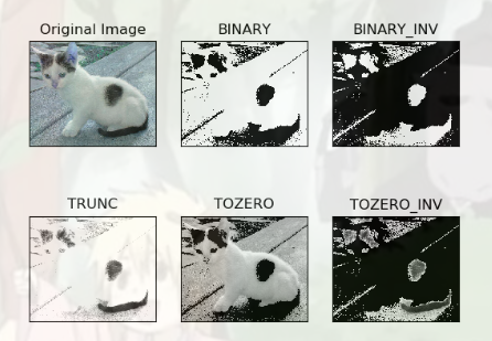
Image Smoothing
1. Mean filter
Simple average convolution operation
Generally, they are odd matrix
blur = cv2.blur(img, (3, 3))
2. Box Filtering
Explanation of parameters:
-1: same color channel
normalize=True: the same effect
normalize=False:>255 assigned to 255
# box filter
# Normalization is optional, just like the mean
box = cv2.boxFilter(img,-1,(3,3), normalize=True)

box = cv2.boxFilter(img,-1,(3,3), normalize=False)
3. Gauss filter
The values in the convolution kernel of a Gaussian blur satisfy the Gaussian distribution, which is equivalent to more emphasis on the middle
The third parameter, the most important of which is set to 1
aussian = cv2.GaussianBlur(img, (5, 5), 1)
4. Median filter
Equivalent to replacing with a median
Complete noise removal
The second parameter: 5 means to find the middle number of the 5*5 matrix
median = cv2.medianBlur(img, 5)
Summary and Contrast Display
import cv2
import numpy as np

img = cv2.imread('img/lenaNoise.png')

# Mean filter
blur = cv2.blur(img, (3, 3))
# box filter
box = cv2.boxFilter(img,-1,(3,3), normalize=False)
# Gauss filter
aussian = cv2.GaussianBlur(img, (5, 5), 1)
# median filtering
median = cv2.medianBlur(img, 5)  # median filtering

# Show All
res = np.hstack((blur,box,aussian,median)) # Horizontal display
# res = np.vstack((blur,box,aussian,median)) # Vertical display
cv2.imshow('median vs average', res)
cv2.waitKey(0)
cv2.destroyAllWindows()
morphology
Corrosion Operation
Iterations: number of iterations
cv2.erode(img,kernel,iterations = 1)
kernel = np.ones((3,3),np.uint8)
erosion = cv2.erode(img,kernel,iterations = 1)
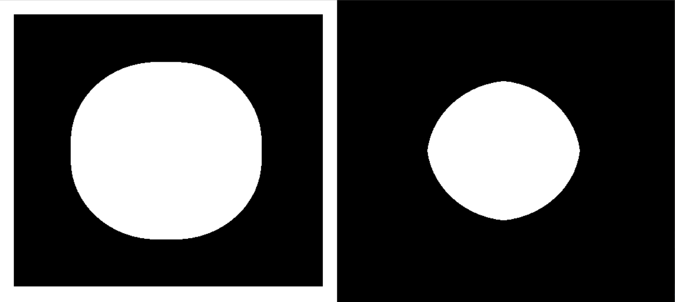
Expansion operation
cv2.dilate(dige_erosion,kernel,iterations = 1)
kernel = np.ones((3,3),np.uint8)
dige_dilate = cv2.dilate(dige_erosion,kernel,iterations = 1)
Open and Closed Operations
On: Corrosion before expansion
cv2.MORPH_OPEN
cv2.morphologyEx(img, cv2.MORPH_OPEN, kernel)
kernel = np.ones((5,5),np.uint8)
opening = cv2.morphologyEx(img, cv2.MORPH_OPEN, kernel)
Closed: Expansion before corrosion
cv2.MORPH_CLOSE
cv2.morphologyEx(img, cv2.MORPH_CLOSE, kernel)
kernel = np.ones((5,5),np.uint8)
cv2.MORPH_CLOSE
closing = cv2.morphologyEx(img, cv2.MORPH_CLOSE, kernel)
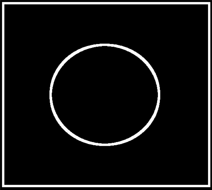
gradient
Gradient=Expansion-Corrosion
cv2.MORPH_GRADIENT
cv2.morphologyEx(pie, cv2.MORPH_GRADIENT, kernel)
# Gradient=Expansion-Corrosion
pie = cv2.imread('img/pie.png')
kernel = np.ones((7,7),np.uint8)

dilate = cv2.dilate(pie,kernel,iterations = 5) # expand
erosion = cv2.erode(pie,kernel,iterations = 5) # corrosion

gradient = cv2.morphologyEx(pie, cv2.MORPH_GRADIENT, kernel) # gradient

res = np.hstack((dilate,erosion,gradient))

cv2.imshow('res', res)
cv2.waitKey(0)
cv2.destroyAllWindows()
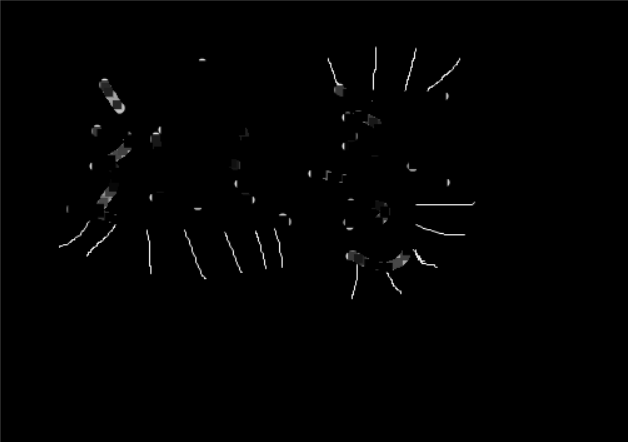
Top hat and black cap
Top hat = original input-open result
cv2.MORPH_TOPHAT
Result: Burrs left behind
tophat = cv2.morphologyEx(img, cv2.MORPH_TOPHAT, kernel)
img = cv2.imread('img/dige.png')
kernel = np.ones((7,7),np.uint8)

tophat = cv2.morphologyEx(img, cv2.MORPH_TOPHAT, kernel)

cv2.imshow('tophat', tophat)
cv2.waitKey(0)
cv2.destroyAllWindows()
Black Cap = Closed Operation - Original Input
Digo Contour
cv2.MORPH_BLACKHAT
cv2.morphologyEx(img,cv2.MORPH_BLACKHAT, kernel)
img = cv2.imread('img/dige.png')
kernel = np.ones((7,7),np.uint8)

blackhat  = cv2.morphologyEx(img,cv2.MORPH_BLACKHAT, kernel)

cv2.imshow('blackhat ', blackhat )
cv2.waitKey(0)
cv2.destroyAllWindows()
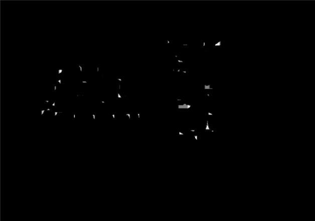
Image Gradient
Sobel Operator
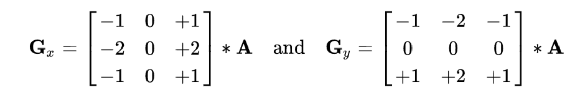
dst = cv2.Sobel(src, ddepth, dx, dy, ksize)
ddepth: The depth of the image
dx and dy represent horizontal and vertical directions, respectively
ksize is the size of the Sobel operator
sobelx = cv2.Sobel(img,cv2.CV_64F,1,0,ksize=3)
tip:
Calculating x,y directly is not recommended because the image will be ghosted
import cv2
import numpy as np

def cv_show(img,name):
    cv2.imshow(name,img)
    cv2.waitKey()
    cv2.destroyAllWindows()

img = cv2.imread('img/pie.png',cv2.IMREAD_GRAYSCALE)

sobelx = cv2.Sobel(img,cv2.CV_64F,1,0,ksize=3)
sobelx = cv2.convertScaleAbs(sobelx)
sobely = cv2.Sobel(img,cv2.CV_64F,0,1,ksize=3)
sobely = cv2.convertScaleAbs(sobely)

sobelxy = cv2.addWeighted(sobelx,0.5,sobely,0.5,0)
cv_show(sobelxy,'sobelxy')
Scharr Operator
Greater weight difference
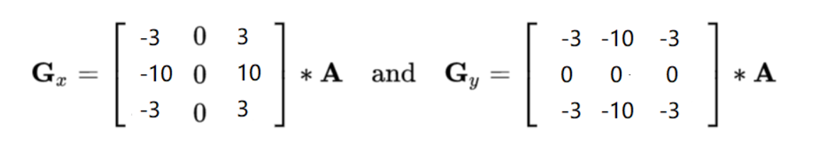
laplacian operator

More sensitive to noise
Usually used with others, not alone
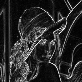
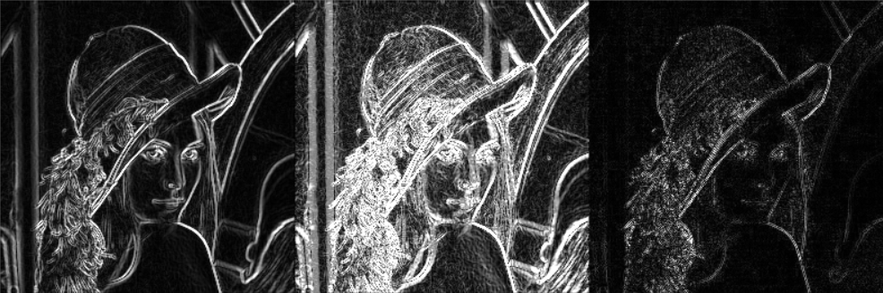
summary
img = cv2.imread('img/lena.jpg',cv2.IMREAD_GRAYSCALE)

#Differences between Operators

sobelx = cv2.Sobel(img,cv2.CV_64F,1,0,ksize=3)
sobely = cv2.Sobel(img,cv2.CV_64F,0,1,ksize=3)
sobelx = cv2.convertScaleAbs(sobelx)
sobely = cv2.convertScaleAbs(sobely)
sobelxy =  cv2.addWeighted(sobelx,0.5,sobely,0.5,0)

scharrx = cv2.Scharr(img,cv2.CV_64F,1,0)
scharry = cv2.Scharr(img,cv2.CV_64F,0,1)
scharrx = cv2.convertScaleAbs(scharrx)
scharry = cv2.convertScaleAbs(scharry)
scharrxy =  cv2.addWeighted(scharrx,0.5,scharry,0.5,0)

laplacian = cv2.Laplacian(img,cv2.CV_64F)
laplacian = cv2.convertScaleAbs(laplacian)

res = np.hstack((sobelxy,scharrxy,laplacian))
cv_show(res,'res')
Canny edge detection
-
Use a Gaussian filter to smooth the image and filter out noise.
-
Calculates the gradient intensity and direction of each pixel point in the image.
-
Non-Maximum Suppression is applied to eliminate the spurious response from edge detection.
-
Double-Threshold detection is applied to determine true and potential edges.
-
Edge detection is finally completed by suppressing isolated weak edges.
img=cv2.imread("img/car.png",cv2.IMREAD_GRAYSCALE)

v1=cv2.Canny(img,120,250)
v2=cv2.Canny(img,50,100) #More detailed

res = np.hstack((v1,v2))
cv_show(res,'res')
image pyramid
1. Gauss Pyramids
Zoom in and zoom out, and the image blurs because there are two losses
Downsampling method (reduced)
img=cv2.imread("AM.png")

down=cv2.pyrDown(img)
cv_show(down,'down')
Upsampling method (amplification)
up=cv2.pyrUp(img)
cv_show(up,'up')
2. Laplacian Pyramids
down=cv2.pyrDown(img)
down_up=cv2.pyrUp(down)
l_1=img-down_up
cv_show(l_1,'l_1')