1. Laplace sharpening

Laplace transform is an integral transform commonly used in engineering mathematics;
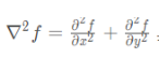
Laplace operator is a second-order differential operator in n-dimensional Euclidean space;

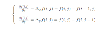
With isotropy, the first derivative of digital image is:

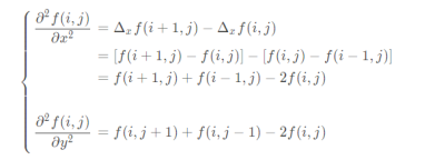
The second derivative is:

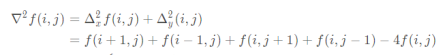
So the Laplace operator is:

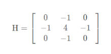
The four neighborhood template of Laplace operator is as follows:

Eight neighborhoods:

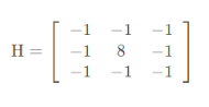
Illustration of convolution:

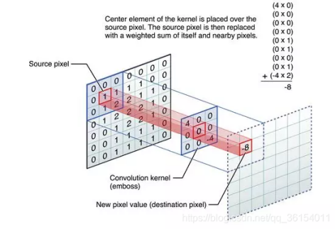
Then, by sliding the convolution kernel, the convolution result of the whole picture can be obtained.

The function of Laplacian edge operator in OpenCV is:

CV_EXPORTS_W void Laplacian( 
InputArray src, 
OutputArray dst, 
int ddepth,
int ksize = 1, 
double scale = 1, 
double delta = 0,
int borderType = BORDER_DEFAULT );

Parameter interpretation:
1. InputArray src: input image

2. OutputArray dst: output image

3. int ddepth: indicates the depth of the output image

4. Depth the bit depth of the image element, which can be one of the following:

Bit depth ---------------------- value range

CV_8U - unsigned 8-bit integer... 0 – 255

CV_8S - signed 8-bit integer... - 128 – 127

CV_16U - unsigned 16 bit integer 0 – 65535

CV_16S - signed 16 bit integer - 32768 – 32767

CV_32S - signed 32-bit integer - 65535 – 65535

CV_32F - single precision floating point number

CV_64F - double precision floating point number
5. int ksize=1: indicates the size of the Laplacian core, and 1 indicates that the size of the core is three:
6. double scale =1: indicates whether to enlarge or reduce the image
7. double delta=0: indicates whether to add an amount to the output pixel
8,int borderType=BORDER_DEFAULT: indicates the method of processing boundaries. It is generally the default

Laplace sharpening steps:
Method 1:
Step 1: use Laplacian edge operator to detect the edge (if it is UCHAR type, negative value shall be reserved):

//The kernel is 0, 1, 0, 1, - 4, 1, 0, 1, 0 		 So the detected edge is negative
cv::Laplacian(src, lapl_1, CV_8U,1,-1);
//The reason for adding a minus sign is to keep the negative number, otherwise the Uchar type directly omits the negative number

Step 2: use the image after the original image and edge detection:

srcaddlapl_1_add = src + lapl_1;//Type must be one to
//It can also be converted to floating-point type (pay attention to normalization) operation, and finally converted to UCHAR type

Method 2: use the image convolution function filter2D()

CV_EXPORTS_W void filter2D( 
InputArray src, 
OutputArray dst, 
int ddepth,
InputArray kernel, 
Point anchor = Point(-1,-1),
double delta = 0, 
int borderType = BORDER_DEFAULT );

Parameter interpretation:
1. InputArray src: input image

2. OutputArray dst: the output image has the same size and number of channels as the input image

3. int ddepth: the depth of the target image. If it is not written, an image with the same depth as the original image will be generated.

The supported depths are as follows (- 1 is the original image depth):
src.depth() = CV_8U,--------------------ddepth = -1/CV_16S/CV_32F/CV_64F
src.depth() = CV_16U/CV_16S, -----ddepth = -1/CV_32F/CV_64F
src.depth() = CV_32F, ------------------ddepth = -1/CV_32F/CV_64F
src.depth() = CV_64F, ------------------ddepth = -1/CV_64F

4. InputArray kernel: convolution kernel (or correlation kernel), a single channel floating-point matrix. If you want to use different kernels in different image channels, you can use the split() function to separate the image channels in advance.

5. Point anchor: the reference point (anchor) of the kernel. Its default value is (- 1, - 1), indicating that it is located in the center of the kernel. The reference point is the point in the kernel that coincides with the pixel point being processed.

6. double delta: the optional value added to the pixel before saving the target image. The default value is 0

7. int borderType: the method of pixel outward approximation. The default value is BORDER_DEFAULT, that is, calculate all boundaries.

Convolution kernel:

cv::Mat  kernel = (cv::Mat_<float>(3, 3) << 0, -1, 0, -1, 5, -1, 0, -1, 0);
//Mat_ Types are used to simplify code

Laplace edge detection operator:

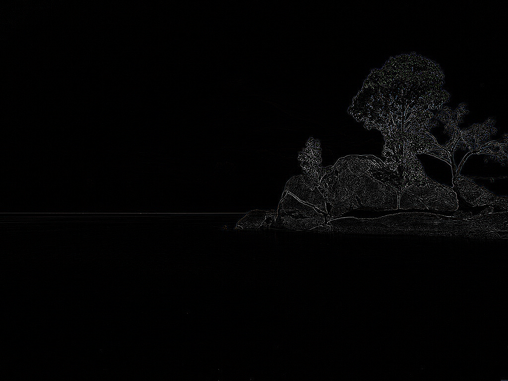
Laplace sharpening operator:

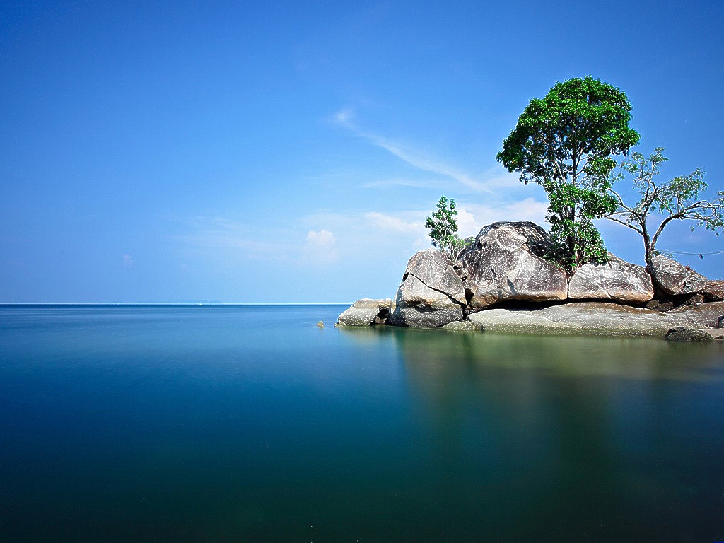
2. Logarithmic transformation

Formula:

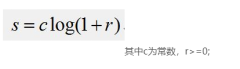
Logarithmic transformation can expand the low gray value part of the image, show more details of the low gray value part, compress the high gray value part and reduce the details of the high gray value part, so as to achieve the purpose of emphasizing the low gray part of the image.

Steps:

//log contrast enhancement
	cv::Mat   src_log(src.size(),CV_64FC3);
	for (int i = 0; i< src.rows;i++)
	{
		for (int j = 0; j< src.cols;j++)
		{
			src_log.at<cv::Vec3d>(i, j)[0] = log(1 + src.at<cv::Vec3b>(i, j)[0]);
			src_log.at<cv::Vec3d>(i, j)[1] = log(1 + src.at<cv::Vec3b>(i, j)[1]);
			src_log.at<cv::Vec3d>(i, j)[2] = log(1 + src.at<cv::Vec3b>(i, j)[2]);

		}

	}
	//The normalization here is because src is not normalized, and the resulting log value is greater than 1. When multiplied by 255, the value will be very large
	normalize(src_log, src_log, 0, 255,cv::NORM_MINMAX,CV_8UC3);
	cv::imshow("src_log", src_log);

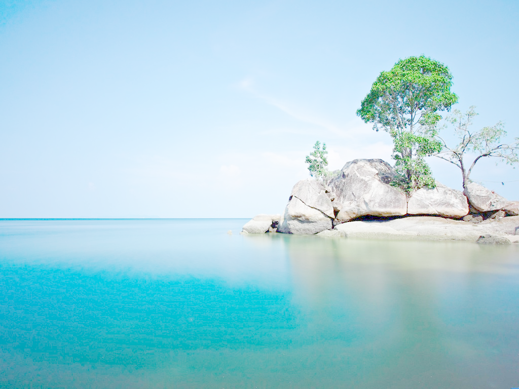
Logarithmic transformation result:

3. Histogram equalization

Histogram equalization formula:

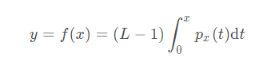
Where f(x) is the function value after equalization,

L is max pixel level,

Is the distribution function of the probability density function,

Is the number of pixels with pixel level x / the total number of pixels.

Theoretical basis:

If an image occupies all possible gray levels and is evenly distributed. Then the image has high contrast and changeable gray tones. Reflected in the image, the details are particularly rich and the image looks high quality.

Steps:
1. Count the number of occurrences of each gray level in the histogram;
2. Cumulative normalized histogram. In the cumulative histogram, the original values with similar probability will be treated as the same value.
3. Calculates a new pixel value.

There are two difficult questions: one is why the cumulative distribution function is selected, and the other is why the pixel values will be evenly distributed after using the cumulative distribution function.

First question. In the process of equalization, two conditions must be guaranteed:

① No matter how the pixels are mapped, we must ensure that the original size relationship remains unchanged. The brighter areas are still brighter, and the darker areas are still darker, but the contrast increases, and the light and shade must not be reversed;
② If it is an eight bit image, the value range of the pixel mapping function should be between 0 and 255 and cannot exceed the limit. Combining the above two conditions, the cumulative distribution function is a good choice, because the cumulative distribution function is a monotonic increasing function (control size relationship) and the value range is 0 to 1 (control out of bounds problem), so the cumulative distribution function is used in histogram equalization.

Second question. Cumulative distribution function has some good properties, so how to use cumulative distribution function to make histogram equalization?

Comparing the probability distribution function with the cumulative distribution function, the two-dimensional image of the former is uneven, and the latter is monotonically increasing.

Use the encapsulated function equalizeHist() in OpenCV;

CV_EXPORTS_W void equalizeHist( InputArray src, OutputArray dst );

Parameter interpretation:
1. InputArray src input image;
2. OutputArray dst output image;
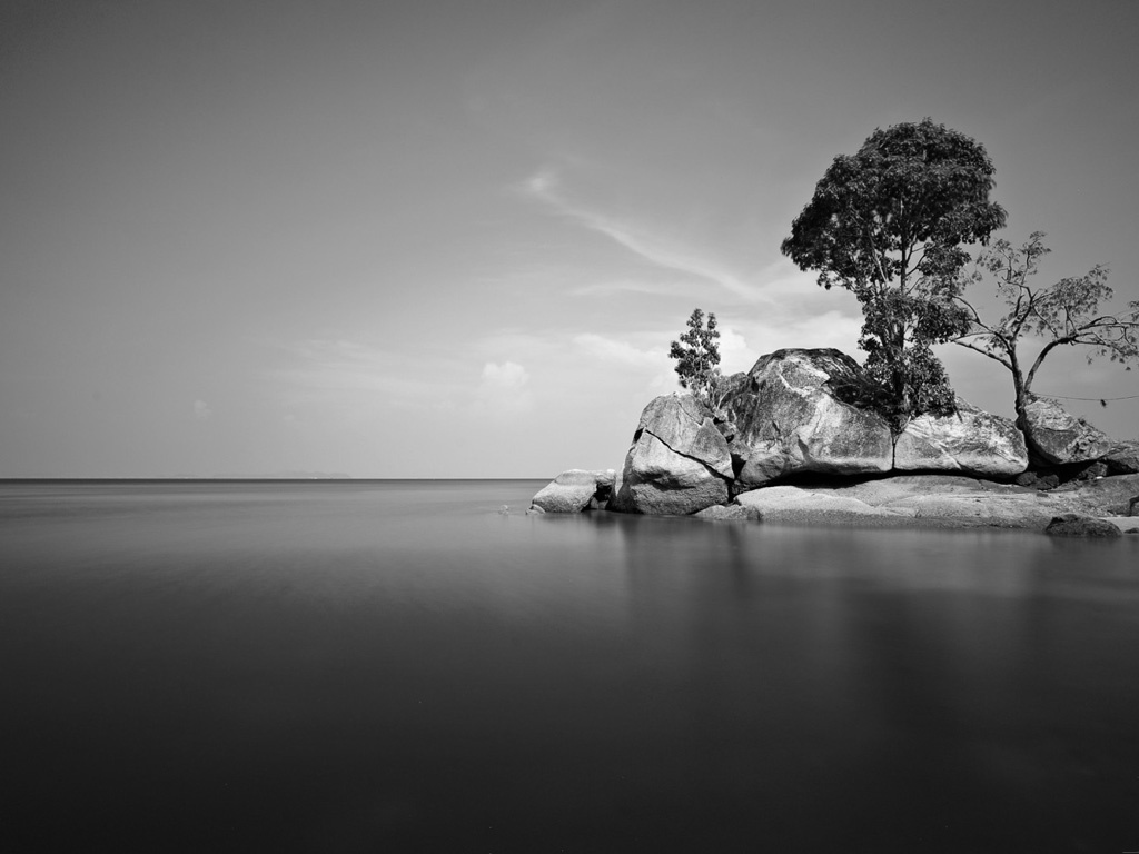
Original grayscale image:

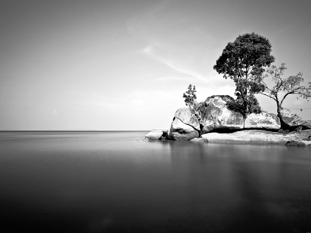
Histogram equalization result (gray single channel):

4. Gamma correction

The formula of gamma transformation is:
s = C r γ s=C r^{\gamma} s=Crγ
s is the pixel value of the transformed image, C is the gray scale coefficient, usually 1, and r is the pixel value of the original image, γ {\gamma } γ Gamma factor controls the scaling degree of the whole algorithm. Gamma transform is also called power transform.

Note: the value range of r is [0,1], so it is necessary to convert the uchar data to float data and normalize it.

cv::Mat::convertTo(dst, CV_32FC3, 1 / 255.0);
//Where dst is the target graph, CV_32FC3 is the type to convert

In the color space represented by integers, the numerical range is 0-255, but in the color space represented by floating-point numbers, the numerical range is 0-1.0, so 0-255 should be normalized.
CV_ The grayscale of 8uc3 or the color component of BGR image are between 0 and 255. imshow can display images directly.
CV_ The value range of 32fc3 is 0 ~ 1.0. When imshow, the image will be displayed after x255.
imwrite cannot save pictures of floating point type.

#include <opencv.hpp>


void main()
{
	cv::Mat src = cv::imread("C:/Users/Administrator/Desktop/test.jpg");

	cv::Mat dst,gamma;
	src.convertTo(dst, CV_32FC3,(double) 1 / 255);
	

	float ga = 0.5;
	cv::pow(dst,ga, gamma);

	
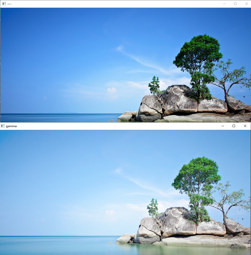
	cv::imshow("src", src);
	cv::imshow("dst",dst);
	cv::imshow("gamma", gamma);
	cv::waitKey(0);
}

As shown in the figure:

Code appendix:

#include <opencv.hpp>



void main()
{
	cv::Mat src = cv::imread("C:/Users/Administrator/Desktop/test.jpg");
	cv::Mat dst,dst_lap, gray,gamma, equal, 
	lapl,lapl_1,src_lap, srcaddlapl_1_add,srcaddlapl_add, srcaddlapl_f_add;

	/*
	dst:CV_32F Type, gamma transform source diagram;
	dst_lap: CV_32F Type, Laplace transform source graph;
	gamma: CV_32F Type, gamma transform output image;
	gray: CV_8UC1 Type, grayscale;
	equal: CV_8UC1 Type, histogram equalization image;
	lapl: Laplacian Image after function convolution;
	src_lap: The image obtained by directly using Laplace sharpening operator to operate the original image;
	srcaddlapl_add: Laplacian The image obtained by the function is calculated with the original image;
	srcaddlapl_1_add: CV_8U Type, scale multiplied by - 1 is converted to UCHAR type without omitting negative numbers;
	srcaddlapl_f_add: The image added to the original image after convolution by Laplace edge operator;
	*/

	cv::cvtColor(src, gray, cv::COLOR_BGR2GRAY);
	src.convertTo(dst, CV_32F, (double)1 / 255);
	src.convertTo(dst_lap, CV_32F, (double)1 / 255);
	/*lapl.convertTo(lapl, CV_64F);*/

	//gamma transform
	double gm = 27 / 40.0;
	cv::pow(dst, gm, gamma);

	//histogram equalization 
	cv::equalizeHist(gray, equal);

	//Laplace transform (kernel is 0, 1, 0, 1, - 4, 1, 0, 1, 0)
	cv::Laplacian(src, lapl_1, CV_8U,1,-1);//The reason for the minus sign is to keep the negative number,
	//Otherwise, the Uchar type directly omits negative numbers

	srcaddlapl_1_add = src + lapl_1;

	cv::Laplacian(dst_lap, lapl, CV_32F);
	cv::imshow("dst_lap", dst_lap);
	cv::imshow("lapl", lapl);
	cv::imshow("lapl_1", lapl_1);
	srcaddlapl_add = dst_lap - lapl;



	//Difference between Laplacian edge detection operator and original image addition and Laplacian sharpening operator
	cv::Mat test_lap,test_src;
	cv::Mat  kernel_1 = (cv::Mat_<float>(3, 3) << 0, -1, 0, -1, 4, -1, 0, -1, 0);
	cv::filter2D(src, test_lap, CV_8U, kernel_1);
	cv::Mat  kernel_2 = (cv::Mat_<float>(3, 3) << 0,0,0,0,1,0,0,0,0);
	cv::filter2D(src, test_src, CV_8U, kernel_2);
	srcaddlapl_f_add = test_src + test_lap  ;
	
	

	//laplacian sharpening 
	cv::Mat  kernel = (cv::Mat_<float>(3, 3) << 0, -1, 0, -1, 5, -1, 0, -1, 0);
	cv::filter2D(src, src_lap, CV_8UC3, kernel);
	
	
	
	//log contrast enhancement
	cv::Mat   src_log(src.size(),CV_64FC3);
	for (int i = 0; i< src.rows;i++)
	{
		for (int j = 0; j< src.cols;j++)
		{
			src_log.at<cv::Vec3d>(i, j)[0] = log(1 + src.at<cv::Vec3b>(i, j)[0]);
			src_log.at<cv::Vec3d>(i, j)[1] = log(1 + src.at<cv::Vec3b>(i, j)[1]);
			src_log.at<cv::Vec3d>(i, j)[2] = log(1 + src.at<cv::Vec3b>(i, j)[2]);

		}

	}
	//The normalization here is because src is not normalized, and the resulting log value is greater than 1. When multiplied by 255, the value will be very large
	normalize(src_log, src_log, 0, 255,cv::NORM_MINMAX,CV_8UC3);
	cv::imshow("src_log", src_log);
	


	cv::imshow("src", src);
	cv::imshow("lapl", lapl);	
	cv::imshow("gamma", gamma);
	cv::imshow("equal", equal);
	cv::imshow("src_lap", src_lap);
	cv::imshow("test_src", test_src);
	cv::imshow("srcaddlapl_add", srcaddlapl_add);
	cv::imshow("srcaddlapl_f_add", srcaddlapl_f_add);
	cv::imshow("srcaddlapl_1_add", srcaddlapl_1_add);
	cv::waitKey(0);
}