Fourier concept

Introduction to Fourier

• Fourier transform, which means that a function satisfying certain conditions can be expressed as a trigonometric function (sine and / or cosine function) or a linear combination of their integrals. In different research fields, Fourier transform has many different variants, such as Continuous Fourier transform and discrete Fourier transform. Initially, Fourier analysis was proposed as a tool for analytical analysis of thermal processes. (refer to Baidu Encyclopedia).
• Generally speaking, we live in a world of time. We get up at 7:00 in the morning, have breakfast at 7:30, go to school at 8:00, finish class at 12:00 and so on. Taking time as a reference is time domain analysis. But in the frequency domain, everything is static! You can refer to this link The concept of Fourier can be understood in a popular way.

Function of Fourier transform

• The role of Fourier in OpenCV:
  • High frequency: grayscale components that change dramatically, such as boundaries.
  • Low frequency: a gray component that changes slowly, such as a sea.

Fourier filtering

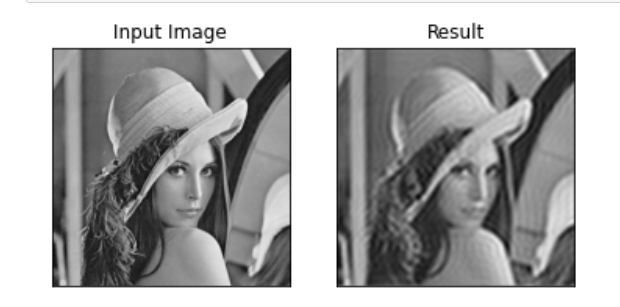
• Low pass filter: only low frequency (gentle amplitude) is retained, which will blur the image.
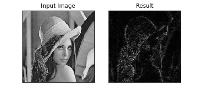
• High pass filter: only high frequency is reserved (the amplitude is intense), which will enhance the image details.

Practical application of OpenCV Fourier transform

Function introduction

• opencv mainly includes cv2.dft() and cv2.idft(). The input image needs to be converted into np.float32 format first.
• In the obtained results, the part with frequency 0 will be in the upper left corner, which usually needs to be converted to the central position, which can be realized by shift transformation.
• The result returned by cv2.dft() is dual channel (real part and imaginary part), which usually needs to be converted into image format to display (0255).

Code presentation

• Conversion form

import numpy as np
import cv2
from matplotlib import pyplot as plt

img = cv2.imread('lena.jpg',0)
img_float32 = np.float32(img)

dft = cv2.dft(img_float32, flags = cv2.DFT_COMPLEX_OUTPUT)
dft_shift = np.fft.fftshift(dft)
# Get the form that the gray image can represent
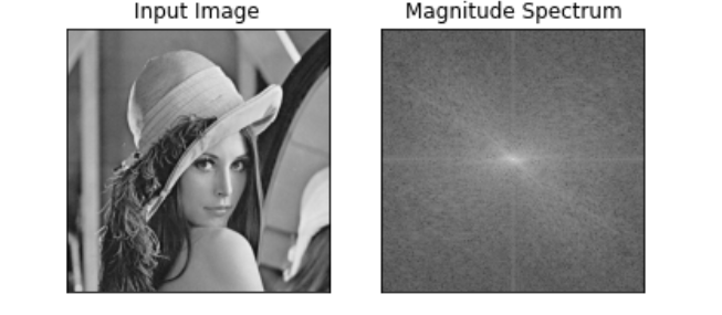
magnitude_spectrum = 20*np.log(cv2.magnitude(dft_shift[:,:,0],dft_shift[:,:,1]))

plt.subplot(121),plt.imshow(img, cmap = 'gray')
plt.title('Input Image'), plt.xticks([]), plt.yticks([])
plt.subplot(122),plt.imshow(magnitude_spectrum, cmap = 'gray')
plt.title('Magnitude Spectrum'), plt.xticks([]), plt.yticks([])
plt.show()

• Low pass filtering effect display

import numpy as np
import cv2
from matplotlib import pyplot as plt

img = cv2.imread('lena.jpg',0)
img_float32 = np.float32(img)

dft = cv2.dft(img_float32, flags = cv2.DFT_COMPLEX_OUTPUT)
dft_shift = np.fft.fftshift(dft)

rows, cols = img.shape
crow, ccol = int(rows/2) , int(cols/2)     # Center position

# Low pass filtering: when outputting detailed features, the outline will appear blurred. When creating a mask, it needs to be centered to 1 and surrounded by a mask matrix of 0.
mask = np.zeros((rows, cols, 2), np.uint8)
mask[crow-30:crow+30, ccol-30:ccol+30] = 1

# IDFT
fshift = dft_shift*mask
f_ishift = np.fft.ifftshift(fshift)
img_back = cv2.idft(f_ishift)
img_back = cv2.magnitude(img_back[:,:,0],img_back[:,:,1])

plt.subplot(121),plt.imshow(img, cmap = 'gray')
plt.title('Input Image'), plt.xticks([]), plt.yticks([])
plt.subplot(122),plt.imshow(img_back, cmap = 'gray')
plt.title('Result'), plt.xticks([]), plt.yticks([])

plt.show()

• High pass filtering effect display

img = cv2.imread('lena.jpg',0)
img_float32 = np.float32(img)

dft = cv2.dft(img_float32, flags = cv2.DFT_COMPLEX_OUTPUT)
dft_shift = np.fft.fftshift(dft)

rows, cols = img.shape
crow, ccol = int(rows/2) , int(cols/2)     # Center position

# High pass filtering: output contour features, remove details, and create a mask matrix centered at 0 and surrounded by 1.
mask = np.ones((rows, cols, 2), np.uint8)
mask[crow-30:crow+30, ccol-30:ccol+30] = 0

# IDFT
fshift = dft_shift*mask
f_ishift = np.fft.ifftshift(fshift)
img_back = cv2.idft(f_ishift)
img_back = cv2.magnitude(img_back[:,:,0],img_back[:,:,1])

plt.subplot(121),plt.imshow(img, cmap = 'gray')
plt.title('Input Image'), plt.xticks([]), plt.yticks([])
plt.subplot(122),plt.imshow(img_back, cmap = 'gray')
plt.title('Result'), plt.xticks([]), plt.yticks([])

plt.show()