Opencv advanced super resolution based on OpenCV

Keywords: Python C++ OpenCV Deep Learning

brief introduction

Super resolution refers to the process of enlarging or improving image details. When increasing the size of the image, additional pixels need to be interpolated in some way. Traditional image processing techniques can not get good results because they do not take the surrounding environment as the background when zooming in. Deep learning and recent GANs play a role here and provide better results.

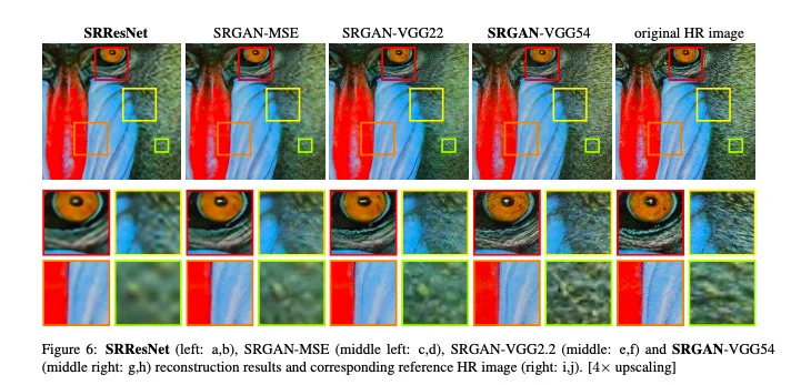
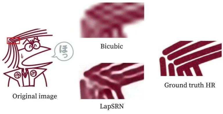
The image given below illustrates the super-resolution. After zooming in, the original high-resolution image shows the best details. Other images are reconstructed by various super-resolution methods. You can here Read more details.

1. Super resolution of opencv

For image scaling, opencv currently has four depth learning algorithms to choose from. In this article, we will review all these methods. We will also see their results and compare them with images scaled using the bicubic interpolation method in OpenCV. The four methods we will discuss are (1) EDSR Model(2)ESPCN Model(3)FSRCNN Model(4)LapSRN Model
Note that the first three algorithms provide ratios of 2, 3, and 4 times, while the last algorithm has 2, 4, and 8 times the original size! The TensorFlow model for each required ratio can be downloaded through the link provided above.

In order to achieve super-resolution using the models listed above, we need to use functions outside the standard OpenCV module. This is why we also have to install the OpenCV contrib module. In addition, super-resolution appears in the module DNN_ In superres (super-resolution based on deep neural network), this module is implemented in OpenCV4.1 of C + + and OpenCV4.3 of Python.

Note: if you already have opencv installed, it's best to create a virtual environment and install opencv contrib in it to avoid any dependency problems. By default, this installs the latest version of OpenCV and the opencv contrib module. If you have installed opencv before running this command, you can also choose to uninstall it.
Code address:

Link: https://pan.baidu.com/s/1M0l63vxYbS7zrF3Pn9IYaQ 
Extraction code: 123 a

In order to compare the above algorithms, we will use the following pictures as a reference.

(1)Python

import cv2
import matplotlib.pyplot as plt
# Read picture
img = cv2.imread("AI-Courses-By-OpenCV-Github.png")
plt.imshow(img[:,:,::-1])
plt.show()
# Crop OpenCV logo
img = img[5:60,700:755]
plt.imshow(img[:,:,::-1])
plt.show()

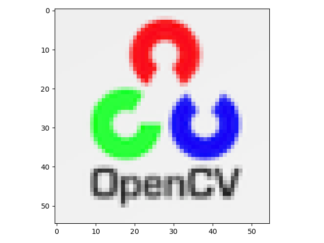
We first import opencv and matplotlib and read the test images. To crop the opencv logo, we use the code given above.
(2)C++

#include <iostream>
#include <fstream>
#include <opencv2/opencv.hpp>
#include <opencv2/dnn_superres.hpp>

using namespace std;
using namespace cv;
using namespace dnn;

// Read picture
Mat img = imread("AI-Courses-By-OpenCV-Github.png");
// Crop region of interest
Rect roi;
roi.x = 700;
roi.y = 5;
roi.width = 55;
roi.height = 55;
img = img(roi);
imshow("roi", img);
cv2.waitKey();
cv2.destroyAllWindows();
return;

2.EDSR

Lim et al. Proposed two methods in their paper, EDSR and MDSR. In EDSR method, different scales need different models. In contrast, in the MDSR model, a single model can reconstruct different scales. However, in this article, we only discuss EDSR.

It uses a ResNet style architecture without batch normalization layer. They found that removing the BN layer can improve performance. This allows them to build larger models with better performance. In order to overcome the instability found in large models, they used a residual scaling factor of 0.1 in each residual block by placing a constant scaling layer after the last convolution layer. In addition, the ReLU activation layer is not used after the residual block.

The architecture was initially trained with a scale factor of 2. These pre trained weights are then used when the training scale factors are 3 and 4. This not only accelerates the training, but also improves the performance of the model. The following figure shows the comparison between the 4x super-resolution results of EDSR method and bicubic interpolation method and the original high-resolution image.

(1)Python

import cv2
import matplotlib.pyplot as plt
# Read picture
img = cv2.imread("AI-Courses-By-OpenCV-Github.png")
img = img[5:60,700:755]
sr = cv2.dnn_superres.DnnSuperResImpl_create()
path = "EDSR_x4.pb"
sr.readModel(path)
sr.setModel("edsr",4)
result = sr.upsample(img)
# Resize image
resized = cv2.resize(img,dsize=None,fx=4,fy=4)
plt.figure(figsize=(12,8))
plt.subplot(1,3,1)
# original image 
plt.imshow(img[:,:,::-1])
plt.subplot(1,3,2)
# SR up sampling image
plt.imshow(result[:,:,::-1])
plt.subplot(1,3,3)
# Sampling images on OpenCV
plt.imshow(resized[:,:,::-1])
plt.show()

(2)C++

#include <iostream>
#include <opencv2/dnn_superres.hpp>
#include <opencv2/imgproc.hpp>
#include <opencv2/highgui.hpp>

using namespace std;
using namespace cv;
using namespace dnn;
using namespace dnn_superres;

Mat upscaleImage(Mat img, string modelName, string modelPath, int scale){
	DnnSuperResImpl sr;
	sr.readModel(modelPath);
	sr.setModel(modelName,scale);
	// Output picture
	Mat outputImage;
	sr.upsample(img, outputImage);
	return outputImage;
}

int main(int argc, char *argv[])
{
	// Read picture
	Mat img = imread("AI-Courses-By-OpenCV-Github.png");
	// Crop region of interest
	Rect roi;
	roi.x = 700;
	roi.y = 5;
	roi.width = 55;
	roi.height = 55;
	img = img(roi);

	// EDSR (x4)
	string path = "EDSR_x4.pb";
	string modelName = "edsr";
	int scale = 4;
	Mat result = upscaleImage(img, modelName, path, scale);

	// Sampling with OpenCV
	Mat resized;
	cv::resize(img, resized, cv::Size(), scale, scale);

	imshow("Original image",img);
	imshow("SR upscaled",result);
	imshow("OpenCV upscaled",resized);
	waitKey(0);
	destroyAllWindows();

	return 0;
}

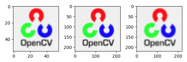
( Left ) primary beginning chart image ， ( in ) E D S R 4 times discharge large chart image ， ( right ) chart image send use O p e n C V of r e s i z e letter number discharge large (left) original image, (middle) edsr4x enlarged image, and (right) image is enlarged using the resize function of OpenCV (left) original image, (middle) edsr4x enlarged image, and (right) image is enlarged using the resize function of OpenCV

3.ESPCN

Shi et al. Did not use the bicubic filter to scale up the low resolution for super-resolution, but extracted the feature map in the low resolution itself and used the complex scale up filter to obtain the results. The upper sampling layer is only deployed at the end of the network. This ensures that complex operations in the model occur in lower dimensions, which makes it faster, especially compared with other technologies.

The basic structure of ESPCN is inspired by SRCNN. Instead of the traditional convolution layer, sub-pixel convolution layer is used, which is similar to deconvolution layer. The last layer uses the sub-pixel convolution layer to generate a high-resolution image. At the same time, they found that the Tanh activation function was much better than the standard ReLU activation function.

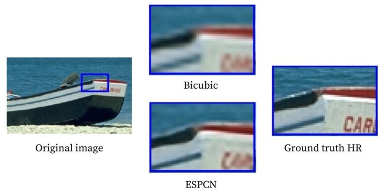
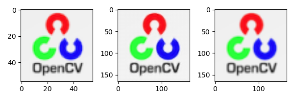
The following figure shows the comparison of 3x super-resolution results of ESPCN method, bicubic interpolation method and original high-resolution image.

(1)Python

import cv2
import matplotlib.pyplot as plt
# Read picture
img = cv2.imread("AI-Courses-By-OpenCV-Github.png")
img = img[5:60,700:755]
sr = cv2.dnn_superres.DnnSuperResImpl_create()
path = "ESPCN_x3.pb"
sr.readModel(path)
sr.setModel("espcn",3)
result = sr.upsample(img)
# Resize image
resized = cv2.resize(img,dsize=None,fx=3,fy=3)
plt.figure(figsize=(6,2))
plt.subplot(1,3,1)
# original image 
plt.imshow(img[:,:,::-1])
plt.subplot(1,3,2)
# SR up sampling image
plt.imshow(result[:,:,::-1])
plt.subplot(1,3,3)
# Sampling images on OpenCV
plt.imshow(resized[:,:,::-1])
plt.show()

(2)C++

#include <iostream>
#include <opencv2/dnn_superres.hpp>
#include <opencv2/imgproc.hpp>
#include <opencv2/highgui.hpp>

using namespace std;
using namespace cv;
using namespace dnn;
using namespace dnn_superres;

Mat upscaleImage(Mat img, string modelName, string modelPath, int scale){
	DnnSuperResImpl sr;
	sr.readModel(modelPath);
	sr.setModel(modelName,scale);
	// Output image
	Mat outputImage;
	sr.upsample(img, outputImage);
	return outputImage;
}

int main(int argc, char *argv[])
{
	// Read picture
	Mat img = imread("AI-Courses-By-OpenCV-Github.png");
	// Crop region of interest
	Rect roi;
	roi.x = 700;
	roi.y = 5;
	roi.width = 55;
	roi.height = 55;
	img = img(roi);

	// ESPCN (x3)
	string path = "ESPCN_x3.pb";
	string modelName = "espcn";
	int scale = 3;
	Mat result = upscaleImage(img, modelName, path, scale);

	// Resizing images using OpenCV
	Mat resized;
	cv::resize(img, resized, cv::Size(), scale, scale);

	imshow("Original image",img);
	imshow("SR upscaled",result);
	imshow("OpenCV upscaled",resized);
	waitKey(0);
	destroyAllWindows();

	return 0;
}

( Left ) primary beginning chart image ， ( in ) E S P C N x 3 rise level chart image ， ( right ) chart image send use O p e n C V of r e s i z e letter number discharge large (left) original image, (middle) ESPCN_x3 upgrade image, (right) the image is enlarged using the resize function of OpenCV (left) original image, (middle) ESPCNx#3 upgraded image, (right) image is enlarged by using the resize function of OpenCV

4.FSRCNN

FSRCNN and ESPCN have very similar concepts. Their basic structure is inspired by SRCNN, and the upper sampling layer is adopted at the end to improve the speed, rather than inserting it early. In addition, they even reduce the input feature dimension, use smaller filter size, and finally use more mapping layers, which makes the model smaller and faster.

The following figure shows the comparison of 3x super-resolution results of FSRCNN method, bicubic interpolation method and original high-resolution image.

(1)Python

import cv2
import matplotlib.pyplot as plt
# Read picture
img = cv2.imread("AI-Courses-By-OpenCV-Github.png")
img = img[5:60,700:755]
sr = cv2.dnn_superres.DnnSuperResImpl_create()
path = "FSRCNN_x3.pb"
sr.readModel(path)
sr.setModel("fsrcnn",3)
result = sr.upsample(img)
# Resize image
resized = cv2.resize(img,dsize=None,fx=3,fy=3)
plt.figure(figsize=(6,2))
plt.subplot(1,3,1)
# original image 
plt.imshow(img[:,:,::-1])
plt.subplot(1,3,2)
# SR up sampling image
plt.imshow(result[:,:,::-1])
plt.subplot(1,3,3)
# Sampling images on OpenCV
plt.imshow(resized[:,:,::-1])
plt.show()

(2)C++

#include <iostream>
#include <opencv2/dnn_superres.hpp>
#include <opencv2/imgproc.hpp>
#include <opencv2/highgui.hpp>

using namespace std;
using namespace cv;
using namespace dnn;
using namespace dnn_superres;

Mat upscaleImage(Mat img, string modelName, string modelPath, int scale){
	DnnSuperResImpl sr;
	sr.readModel(modelPath);
	sr.setModel(modelName,scale);
	// output
	Mat outputImage;
	sr.upsample(img, outputImage);
	return outputImage;
}

int main(int argc, char *argv[])
{
	// Read picture
	Mat img = imread("AI-Courses-By-OpenCV-Github.png");
	// Crop ROI
	Rect roi;
	roi.x = 850;
	roi.y = 0;
	roi.width = img.size().width - 850;
	roi.height = 80;
	img = img(roi);

	// FSRCNN (x3)
	string path = "FSRCNN_x3.pb";
	string modelName = "fsrcnn";
	int scale = 3;
	Mat result = upscaleImage(img, modelName, path, scale);

	// Resizing images using OpenCV
	Mat resized;
	cv::resize(img, resized, cv::Size(), scale, scale);

	imshow("Original image",img);
	imshow("SR upscaled",result);
	imshow("OpenCV upscaled",resized);
	waitKey(0);
	destroyAllWindows();
	return 0;
}

( Left ) primary beginning chart image ， in ( ) F S R C N N _ 3 times of discharge large chart image ， ( right ) send use O p e n C V of r e s i z e letter number discharge large chart image (left) original image, middle (fsrcnn)\_ Enlarge the image by 3x, (right) use the resize function of OpenCV to enlarge the image (left) original image, middle (fsrcnn)_ Enlarge the image by 3x, (right) use the resize function of OpenCV to enlarge the image

5.LapSRN

Lapsrn provides a middle ground in the start and end comparison strategy. It recommends gentle sampling until the end. Its name is based on the Laplacian pyramid. Its structure is basically like a pyramid, which is constantly upgraded on low resolution images until the end. For speed, parameter sharing is very dependent; Like the EDSR model the first mock exam is a single model that can be rebuilt at different scales, called MS-LapSRN. However, in this article, we only discuss lapsrn.

The model includes two branches: feature extraction and image reconstruction. There is parameter sharing between different scales, such as 4x using the parameters of the 2x model. This means one pyramid for scaling 2x, two for scaling 4x, and three for scaling 8x! Making such depth models means that they may encounter the problem of gradient disappearance. Therefore, they try different types of local hop connections, such as different source hop connections and shared source connections. The loss function of the model uses charbonier loss and does not use batch normalization layer.

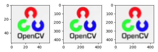
The following figure shows the comparison between the 8x super-resolution results of LapSRN method and bicubic interpolation method and the original high-resolution image.

(1)Python

import cv2
import matplotlib.pyplot as plt
# Read picture
img = cv2.imread("AI-Courses-By-OpenCV-Github.png")
img = img[5:60,700:755]
sr = cv2.dnn_superres.DnnSuperResImpl_create()
path = "LapSRN_x8.pb"
sr.readModel(path)
sr.setModel("lapsrn",8)
result = sr.upsample(img)
# Resize image
resized = cv2.resize(img,dsize=None,fx=8,fy=8)
plt.figure(figsize=(6,2))
plt.subplot(1,3,1)
# original image 
plt.imshow(img[:,:,::-1])
plt.subplot(1,3,2)
# SR up sampling image
plt.imshow(result[:,:,::-1])
plt.subplot(1,3,3)
# Sampling images on OpenCV
plt.imshow(resized[:,:,::-1])
plt.show()

(2)C++

#include <iostream>
#include <opencv2/dnn_superres.hpp>
#include <opencv2/imgproc.hpp>
#include <opencv2/highgui.hpp>

using namespace std;
using namespace cv;
using namespace dnn;
using namespace dnn_superres;

Mat upscaleImage(Mat img, string modelName, string modelPath, int scale){
	DnnSuperResImpl sr;
	sr.readModel(modelPath);
	sr.setModel(modelName,scale);
	// output
	Mat outputImage;
	sr.upsample(img, outputImage);
	return outputImage;
}

int main(int argc, char *argv[])
{
	// Read picture
	Mat img = imread("AI-Courses-By-OpenCV-Github.png");
	// Crop region of interest
	Rect roi;
	roi.x = 850;
	roi.y = 0;
	roi.width = img.size().width - 850;
	roi.height = 80;
	img = img(roi);

	// LapSRN (x2)
	string path = "LapSRN_x8.pb";
	string modelName = "lapsrn";
	int scale = 8;
	Mat result = upscaleImage(img, modelName, path, scale);

	// Upsampling using OpenCV
	Mat resized;
	cv::resize(img, resized, cv::Size(), scale, scale);

	imshow("Original image",img);
	imshow("SR upscaled",result);
	imshow("OpenCV upscaled",resized);
	waitKey(0);
	destroyAllWindows();

	return 0;
}

6. Comparison of results

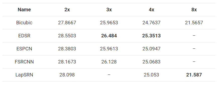
To show the results here, only the butterfly area in the above image has been cropped out. The super-resolution model was used for four magnifications, as shown in the table below.

Python code compared:

import cv2
import matplotlib.pyplot as plt

# Read picture
img = cv2.imread("image.png")
plt.imshow(img[130:290, 150:360, ::-1])
# plt.show()
plt.figure(figsize=(12, 8))
img = img[130:290, 150:360]

# EDSR_x4
sr = cv2.dnn_superres.DnnSuperResImpl_create()
path = "EDSR_x4.pb"
sr.readModel(path)
sr.setModel("edsr", 4)
result_edsr = sr.upsample(img)
plt.subplot(2, 2, 1)
plt.xticks([])
plt.yticks([])
plt.xlabel("EDSR_x4")
plt.imshow(result_edsr[:, :, ::-1])

# ESPCN_x4
sr = cv2.dnn_superres.DnnSuperResImpl_create()
path = "ESPCN_x4.pb"
sr.readModel(path)
sr.setModel("espcn", 4)
result_espcn = sr.upsample(img)
plt.subplot(2, 2, 2)
plt.xticks([])
plt.yticks([])
plt.xlabel("ESPCN_x4")
plt.imshow(result_espcn[:, :, ::-1])

# FSRCNN_x4
sr = cv2.dnn_superres.DnnSuperResImpl_create()
path = "FSRCNN_x4.pb"
sr.readModel(path)
sr.setModel("fsrcnn", 4)
result_fsrcnn = sr.upsample(img)
plt.subplot(2, 2, 3)
plt.xticks([])
plt.yticks([])
plt.xlabel("FSRCNN_x4")
plt.imshow(result_fsrcnn[:, :, ::-1])

# LapSRN_x4
sr = cv2.dnn_superres.DnnSuperResImpl_create()
path = "LapSRN_x4.pb"
sr.readModel(path)
sr.setModel("lapsrn", 4)
result_lapsrn = sr.upsample(img)
plt.subplot(2, 2, 4)
plt.imshow(result_lapsrn[:, :, ::-1])
plt.xticks([])
plt.yticks([])
plt.xlabel("LapSRN_x4")
plt.show()

It is difficult to distinguish different results with the naked eye only by enlarging the image. Therefore, in order to verify the performance of all models, these techniques are applied to three images with a size of 500x333, reduced to the required size, and then sampled back to 500x333. Then, PSNR and SSIM are used to compare the enlarged image with the original image. The average results of all images are calculated, as shown in the figure below.

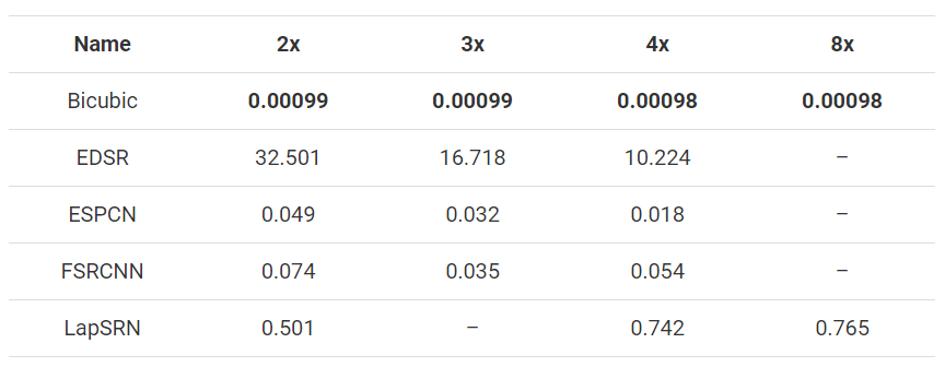
In addition, the time spent on Intel i5-7200U is recorded. The average value of all images is given below. Remember that 3x image size takes less time than 2x, and the same is true if the scaling factor is larger.

(1)Python

import numpy as np
import cv2 as cv
import argparse
import sys


def getPSNR(I1, I2):
    s1 = cv.absdiff(I1, I2)  # |I1 - I2|
    s1 = np.float32(s1)  # Here we use CVs_ 32F, because 8-bit unsigned char cannot be squared
    s1 = s1 * s1  # |I1 - I2|^2
    sse = s1.sum()  # Per channel element and
    if sse <= 1e-10:
        return 0  # Returns 0 for smaller values
    else:
        shape = I1.shape
        mse = 1.0 * sse / (shape[0] * shape[1] * shape[2])
        psnr = 10.0 * np.log10((255 * 255) / mse)
        return psnr


def getMSSISM(i1, i2):
    C1 = 6.5025
    C2 = 58.5225
    # INITS

    I1 = np.float32(i1)  # Cannot calculate on a single byte pixel, the range is not enough.
    I2 = np.float32(i2)

    I2_2 = I2 * I2  # I2^2
    I1_2 = I1 * I1  # I1^2
    I1_I2 = I1 * I2  # I1 * I2
    # END INITS

    # PRELIMINARY COMPUTING
    mu1 = cv.GaussianBlur(I1, (11, 11), 1.5)
    mu2 = cv.GaussianBlur(I2, (11, 11), 1.5)

    mu1_2 = mu1 * mu1
    mu2_2 = mu2 * mu2
    mu1_mu2 = mu1 * mu2

    sigma1_2 = cv.GaussianBlur(I1_2, (11, 11), 1.5)
    sigma1_2 -= mu1_2

    sigma2_2 = cv.GaussianBlur(I2_2, (11, 11), 1.5)
    sigma2_2 -= mu2_2

    sigma12 = cv.GaussianBlur(I1_I2, (11, 11), 1.5)
    sigma12 -= mu1_mu2

    t1 = 2 * mu1_mu2 + C1
    t2 = 2 * sigma12 + C2
    t3 = t1 * t2  # t3 = ((2*mu1_mu2 + C1).*(2*sigma12 + C2))

    t1 = mu1_2 + mu2_2 + C1
    t2 = sigma1_2 + sigma2_2 + C2
    t1 = t1 * t2  # t1 =((mu1_2 + mu2_2 + C1).*(sigma1_2 + sigma2_2 + C2))

    ssim_map = cv.divide(t3, t1)  # ssim_map =  t3./t1;

    mssim = cv.mean(ssim_map)  # mssim = average of ssim map
    return mssim


if __name__ == "__main__":
    # When reading the two input images, ensure that the two images are consistent in size
    img1 = cv.imread('image.jpg')
    img2 = cv.imread('output.jpg')
    img2 = cv.resize(img2, (img1.shape[1],img1.shape[0]))
    print(img1.shape)
    print(img2.shape)
    # Call function
    psnr = getPSNR(img1, img2)
    mssimV = getMSSISM(img1, img2)
    print(psnr)
    print(mssimV)

(2)C++

#include <opencv2/core/core.hpp>
#include <opencv2/highgui/highgui.hpp> 
// The larger the PSNR value between the two images, the more similar it is.
//The input format is Mat type, and I1 and I2 represent the two input images
double getPSNR(const Mat& I1, const Mat& I2)
{
    Mat s1;
    absdiff(I1, I2, s1);       // |I1 - I2|AbsDiff function is a function that calculates the absolute value of the difference between two arrays in OpenCV
    s1.convertTo(s1, CV_32F);  // Here we use CVs_ 32F, because 8-bit unsigned char cannot be squared
    s1 = s1.mul(s1);           // |I1 - I2|^2
    Scalar s = sum(s1);         //Sum each channel
    double sse = s.val[0] + s.val[1] + s.val[2]; // sum channels
    if( sse <= 1e-10) // For very small values, we will be approximately equal to 0
        return 0;
    else
    {
        double  mse =sse /(double)(I1.channels() * I1.total());//Calculate MSE
        double psnr = 10.0*log10((255*255)/mse);
        return psnr;//Return to PSNR
    }
}
Scalar getMSSIM( const Mat& i1, const Mat& i2)
{
	 const double C1 = 6.5025, C2 = 58.5225;
	 /***************************** INITS **********************************/
	 int d = CV_32F;
	 Mat I1, I2;
	 i1.convertTo(I1, d);           // Cannot calculate on a single byte pixel, the range is not enough.
	 i2.convertTo(I2, d);
	
	 Mat I2_2   = I2.mul(I2);        // I2^2
	 Mat I1_2   = I1.mul(I1);        // I1^2
	 Mat I1_I2  = I1.mul(I2);        // I1 * I2
	
	 /***********************Preliminary calculation******************************/
	
	 Mat mu1, mu2;   //Preliminary calculation
	 GaussianBlur(I1, mu1, Size(11, 11), 1.5);
	 GaussianBlur(I2, mu2, Size(11, 11), 1.5);
	
	 Mat mu1_2   =   mu1.mul(mu1);
	 Mat mu2_2   =   mu2.mul(mu2);
	 Mat mu1_mu2 =   mu1.mul(mu2);

	 Mat sigma1_2, sigma2_2, sigma12;
	 GaussianBlur(I1_2, sigma1_2, Size(11, 11), 1.5);
	 sigma1_2 -= mu1_2;
	 GaussianBlur(I2_2, sigma2_2, Size(11, 11), 1.5);
	 sigma2_2 -= mu2_2;
	 GaussianBlur(I1_I2, sigma12, Size(11, 11), 1.5);
	 sigma12 -= mu1_mu2;
	 / formula 
	 Mat t1, t2, t3;
	 t1 = 2 * mu1_mu2 + C1;
	 t2 = 2 * sigma12 + C2;
	 t3 = t1.mul(t2);          // t3 = ((2*mu1_mu2 + C1).*(2*sigma12 + C2))
	
	 t1 = mu1_2 + mu2_2 + C1;
	 t2 = sigma1_2 + sigma2_2 + C2;
	 t1 = t1.mul(t2);   // t1 =((mu1_2 + mu2_2 + C1).*(sigma1_2 + sigma2_2 + C2))
	
	 Mat ssim_map;
	 divide(t3, t1, ssim_map);     // ssim_map =  t3./t1;
	
	 Scalar mssim = mean( ssim_map ); // mssim = ssim_ Average value of map
	 return mssim;
}
int main()
{
	//Define PSNR first
	double psnr;
	//Then read the two input images to ensure that the two images are the same size
	Mat img1=imread('1.jpg');
	Mat img2=imread('2.jpg');
	//Call function
	psnr = getPSNR(img1,img2);  
	mssimV = getMSSIM(img1,img2);
	cout << " PSNR: " << setiosflags(ios::fixed) << setprecision(3) << psnrV << "dB";
	cout << " MSSIM: "
                << " R " << setiosflags(ios::fixed) << setprecision(2) << mssimV.val[2] * 100 << "%"
                << " G " << setiosflags(ios::fixed) << setprecision(2) << mssimV.val[1] * 100 << "%"
                << " B " << setiosflags(ios::fixed) << setprecision(2) << mssimV.val[0] * 100 << "%";
}

When examining the compressed video, this value is about 30 to 50. The larger the number, the better the compression quality. If the image difference is obvious, you may get a value of 15 or even lower. PSNR algorithm is simple and fast. However, the difference value is sometimes out of proportion to people's subjective feelings. Therefore, another algorithm called structural similarity index measure (SSIM) has made improvements in this regard.

SSIM operation will return a similarity for each channel of the image, and the value range should be between 0 and 1. When the value is 1, it means full compliance. However, although SSIM can produce better data, Gaussian blur takes a lot of time, so people still use PSNR algorithm more in a real-time system (24 frames per second).

For this reason, in the initial source code, we use PSNR algorithm to calculate each frame of image, and only when the result calculated by PSNR algorithm is lower than the input value, we use SSIM algorithm to verify.

application

Super-resolution is not only a tool to turn the investigation of science fiction or crime films into reality. Super-resolution is applied in various fields.

Medical Imaging: super resolution is a good solution to improve the quality of x-ray and CT scanning. It helps to highlight important details about human anatomy and function. Improving resolution or enhancing medical images also helps to highlight tumors.
Multimedia, Image, and Video Processing Applications: super resolution can convert blurred frames in mobile phone video into clear and readable images or snapshots.
Biometric Identification: through the enhancement of face, fingerprint and iris images, super-resolution plays a vital role in biometrics. The shape, structure and texture have been greatly enhanced, which is helpful to identify biometric fingerprints.
Remote Sensing: the concept of using super-resolution in Remote Sensing and satellite imaging has been developed for decades. In fact, the first idea of super-resolution was inspired by the demand for higher quality and higher resolution Landsat Remote Sensing images.
Astronomical imaging: improving the resolution of astronomical images helps to pay attention to small details, which may become a major discovery in outer space.
Surveillance Imaging: traffic monitoring and safety system plays a very important role in maintaining civilian safety. The application of super-resolution in digital video recording is very helpful in identifying traffic or safety violations.

summary

In this blog, we briefly introduce the concept of super-resolution. We select four super-resolution models and discuss their architecture and results to highlight the diversity of image super-resolution selection and the efficiency of these methods.

Summarizing our observations, EDSR easily gives the best results of the four methods. However, it is too slow to be used in real-time applications. ESPCN and FSRCNN are the preferred methods for real-time performance and performance. For 8x magnification factor, LapSRN's 8x magnification model performs better in most cases, even if 2x and 4x combined models can be used. Although these methods The speed is not comparable with the traditional bicubic method, but they all have certain advantages.

Reference catalogue

https://blog.csdn.net/yat_chiu/article/details/77893485
https://learnopencv.com/super-resolution-in-opencv/
http://www.opencv.org.cn/opencvdoc/2.3.2/html/doc/tutorials/highgui/video-input-psnr-ssim/video-input-psnr-ssim.html

Posted by MalikBB on Sat, 25 Sep 2021 23:42:13 -0700

Programmer Group

Opencv advanced super resolution based on OpenCV

brief introduction

1. Super resolution of opencv

2.EDSR

3.ESPCN

4.FSRCNN

5.LapSRN

6. Comparison of results

application

summary

Reference catalogue

Hot Keywords