Preface

Due to the influence of many factors in the actual modeling process, its objective function or constraints are difficult to be expressed in a linear relationship. The optimization of such non-linear problems is called a non-linear programming problem, which is basically defined as an extreme value problem of an n-ary function under the constraints of a set of equations or inequalities. At least one of the objective functions and the constraint conditions is a non-linear function of unknown quantities. One-dimensional optimization problems are those in which the poles of a unary function are searched for.

One-dimensional optimization method

When abstracting an actual physical problem into a mathematical model, the following steps are generally followed:

1) Determine the independent variable;

2) Determine optimization objectives;

3) Determine the constraints;

4) Determine the range of independent variables;

The general form of non-linear programming problems can be expressed as:

Where,A decision variable called a model.Called the objective function,andIt is called a constraint function, the former is an equality constraint, the latter is an inequality constraint.

Common one-dimensional optimization methods include golden section method, tangent method, interpolation method, and so on. They basically follow one idea:

From an outletStart in a properly chosen directionSearch (usually as a descent method of the objective function) to get points with smaller target values; Then fromStart, follow the chosen directionSearch for points smaller than the objective function.

How to determine the next optimization direction of the objective function, we use theTo represent. For one-dimensional optimization problems, it is essentially converted to a solution step factorThe extreme value problem of.

The basic steps for one-dimensional search are as follows:

1) Determine the search interval;

2) Determine the extreme point of the function by gradually reducing the interval or approaching the function.

The common methods are forward-backward method, golden section method, Fibonacci method, Newton method, secant method, and so on.

Advance and Retreat Method

The basic idea of the Law of Advance and Retreat refers to:

Single Valley FunctionFor anyIfThenThe search interval for the minimum point; IfThenIs the search interval for the maximum point.

The code examples for the forward and backward methods are as follows for reference only:

function [min_x,max_x]=minJT(f,x0,h0,eps)
% the opotimum method of advance and retreat
% The forward-backward method is an algorithm used to determine the search interval
% The purpose of this custom function is to find the interval of the minimum value
% objective function f
% Initial Point x0
% accuracy eps
if nargin==3
    eps=1E-6;
end
x1=x0;
k=0;
h=h0;
while 1
    x4=x1+h;
    k=k+1;
    f4=subs(f,symvar(f),x4);
    f1=subs(f,symvar(f),x1);
    if f4<f1
        x2=x1;
        x1=x4;
        f2=f1;
        f1=f4;
        h=2*h;
    else
        if k==1
            h=-h;
            x2=x4;
            f2=f4;
        else
            x3=x2;
            x2=x1;
            x1=x4;
            break
        end
    end
end
min_x=min(x1,x3);
max_x=x1+x3-min_x;
end

Golden Section

The basic idea of the golden section method is basically the same as that of the forward-backward method.The following requirements have been made for the value of:

Where,Take 0.618.

The code examples for the golden section method are as follows for reference only:

function [x,minf]=minHJ(f,a,b,N,eps)
% golden section method - Golden Section
% The algorithm works by choosing x1 and x2，Make two points in between[a b]The upper position is symmetrical;
% Simultaneously satisfied, points within the new interval x3 Requires that points already in the interval be symmetrical with respect to the search interval.
% objective function f
% Left Endpoint of Extreme Interval a
% Right Endpoint of Extremum Interval b
% accuracy eps
% Independent variable with minimum objective function x
% Minimum value of objective function minf
if nargin==3
N=10000;
eps=1E-6;
elseif nargin==4
eps=1E-6;
end
l=a+0.382*(b-a);
u=a+0.618*(b-a);
k=1;
tol=b-a;
while tol>eps && k<N
fl=subs(f,symvar(f),l);
fu=subs(f,symvar(f),u);
if fl>fu
a=l;
l=u;
u=a+0.618*(b-a);
else
b=u;
u=l;
l=a+0.382*(b-a);
end
k=k+1;
tol=abs(b-a);
end
if k==N
disp('Minimum value not found')
x=NaN;
minf=NaN;
return
end
x=(a+b)/2;
minf=double(subs(f,symvar(f),x));
end

Fibonacci Law

The Fibonacci method is consistent with the basic idea of the golden section method, but it aims atThe values are different:

WhereIs the nth Fibonacci number.

The code examples for the Fibonacci method are as follows for reference only:

function [min_x,min_s,a,b]=fibonacci(s,a0,b0,eps)
% Fibonacci Law:1,1,2,3,5,8,13,21,34,55,89,......
% When using the Fibonacci method n When a search point is shortened to an interval, the interval length is shortened for the first time to Fn-1/Fn，
% Each subsequent time was Fn-2/Fn-1,Fn-2/Fn-3,......,F1/F2. 
% That is, intervals[a b]Insert Two Points t1，t2，satisfy t1=a+Fn-1/Fn*(b-a)，t2=a+Fn-2/Fn*(b-a)
% objective function f(Symbol expression)
% Left Endpoint of Extreme Interval a0
% Right Endpoint of Extremum Interval b0
% accuracy eps
% Output: Left Endpoint of Split Extremum Interval a
% Output: Right Endpoint of Split Extremum Interval b
% Output: The independent variable corresponding to the minimum value min_x
% Output: Minimum Value min_s
fn=floor((b0-a0)/eps)+1;
f0=1;
f1=1;
n=1;
while f1<fn 
    f2=f1;
    f1=f1+f0;
    f0=f2;
    n=n+1;
end
f=ones(n,1);
for i=2:n
    f(i+1)=f(i)+f(i-1);
end
k=1;
t1=a0+f(n-2)/f(n)*(b0-a0);
t2=a0+f(n-1)/f(n)*(b0-a0);
while k<n-1
    % func4 For a custom function, the target function
    f1=double(subs(s,symvar(s),t1));
    f2=double(subs(s,symvar(s),t2));
    if f1<f2
        b0=t2;
        t2=t1;
        t1=b0+f(n-1-k)/f(n-k)*(a0-b0);
    else
        a0=t1;
        t1=t2;
        t2=a0+f(n-1-k)/f(n-k)*(b0-a0);
    end
    k=k+1;
end
t2=(a0+b0)/2;
t1=a0+(1/2+1E-4)*(b0-a0);
f1=double(subs(s,symvar(s),t1));
f2=double(subs(s,symvar(s),t2));
if f1<f2
    x=t1;
    a=a0;
    b=t1;
else
    x=t2;
    a=t2;
    b=b0;
end
min_x=(a+b)/2;
min_s=double(subs(s,symvar(s),min_x));
end

Newton method

Target functionAt pointAt Tyler:

Assume objective functionAt pointIf the maximum or minimum value is chosen, its first derivative is 0:

The deduction is as follows:

The code examples for the Newton method are as follows for reference only:

function [x,minf]=nwfun(f,x0,accuracy)
% Newton's method: finding the extreme point near the initial point
% Expand the second order Taylor of the objective function and derive it at a point=0，Sequential extremum
% D: x1=x0-inv(Hesse Matrix)*First Order Partial Derivation
% objective function f(Symbol expression)
% Initial Point x0(Column Vector)
% accuracy accuracy
% The value of the independent variable at the minimum of the objective function x
% Minimum value of objective function min_f
if nargin<3
    accuracy=1E-6;
end
InVar=symvar(f);% Get an independent variable Independent Variable
% D1f=zeros(length(InVar),1);
for i=1:length(InVar)
   D1f(i,1)=diff(f,InVar(i));
end
% D2f=zeros(length(InVar),length(InVar));
for i=1:length(InVar)
    for j=1:length(InVar)
        D2f(i,j)=diff(D1f(i),InVar(j));
    end
end
x=x0;
n=0;
while n==0 || norm(g1)>accuracy
g1=zeros(length(D1f),1);
for i=1:length(D1f)
    k=find(InVar==symvar(D1f(i)));
    g1(i,1)=double(subs(D1f(i),symvar(D1f(i)),x(k)'));
end
g2=zeros(size(D2f));
for i=1:length(D1f)
    for j=1:length(D1f)
        k=find(InVar==symvar(D2f(i,j)));
        g2=double(subs(D2f(i,j),symvar(D2f(i,j)),x(k)'));
    end
end
p=-inv(g2)*g1;
x=x+p;
n=n+1;
if n>10000
    disp('10,000 cycles, no results found, please reduce accuracy')
    break
end
end
x=x-p;
minf=double(subs(f,symvar(f),x'));
end

Secant method

The basic idea of secant method is the same as Newton method, but it avoids the process of derivation and inversion of Newton method and speeds up the search efficiency. Its iteration formula is as follows:

The code examples for secant method are as follows for reference only:

function [x,min_f]=minGX(f,x0,x1,accuracy)
% Secant method: suitable for univariate multiorder functions;Find the extreme point near the initial point;
% objective function f(Symbol expression)
% Initial Point x0，x1
% accuracy accuracy
% Independent variable with minimum objective function x
% Minimum value of objective function min_f
if nargin==3
    accuracy=1E-6;
end
d1f=diff(f);
k=0;
tol=1;
while tol>accuracy
    d1fx1=double(subs(d1f,symvar(d1f),x1));
    d1fx0=double(subs(d1f,symvar(d1f),x0));
    x2=x1-(x1-x0)*d1fx1/(d1fx1-d1fx0);
    k=k+1;
    tol=abs(d1fx1);
    x0=x1;
    x1=x2;
end
x=x2;
min_f=double(subs(f,symvar(f),x));
end

One-dimensional optimization using Matlab: fminbnd

The format for calling the fminbnd function of the Matlab command is as follows: (See the mathwork website for details)

x=fminbnd (fun,x1,x2): Returns the minimum value of the objective function fun on an interval [x1,x2];

x=fminbnd (fun,x1,x2,options): Options is the optimization parameter option, which can be set through optimset;

options	Explain
Display	off: No output is displayed; iter: Display information for each iteration; Final: Display the final result;
MaxFunEvals	Maximum number of times allowed for function evaluation
MaxIter	Maximum number of iterations allowed for a function
TolX	Tolerance of x

[x,fval]=fminbnd(...):x is the minimum value returned and Fval is the minimum value of the target function;

[x,fval,exitflag]=fminbnd(...):exitflag is the termination iteration condition with the following values:

exitflag	Explain
1	Indicates that the function converges to solution x
0	Indicates the maximum number of times a function has been evaluated or iterated
-1	Represents the non-convergent solution x of the function
-2	Error in interval indicating input, i.e. X1 > x2

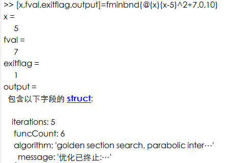
[x,fval,evitflag,output]=fminbnd(...):output is the optimal output information in the form of a structure whose values and descriptions are as follows:

output	Explain
iterations	Represents the number of times the algorithm has fallen
funccount	Represents the number of times a function is assigned
algorithm	Represents the algorithm used to solve linear programming problems
message	Information indicating the termination of the algorithm

Example 01:

Solve the following optimization problems:

Set up the Matlab command stream as needed, as follows:

[x,fval,exitflag,output]=fminbnd(@(x)(x-5)^2+7,0,10)

The results are as follows: