Interpolation is different from fitting. The interpolation function passes through the sample points, and the fitting function is generally based on the least square method as close as possible to all sample points. The common interpolation methods are Lagrange interpolation, piecewise interpolation and spline interpolation.

1. Lagrange Interpolation Polynomials: when the number of nodes n is large, the degree of Lagrange interpolation polynomials is high, inconsistent convergence may occur, and the calculation is complex. With the increase of sample points, the vibration phenomenon that high order interpolation will bring errors is called Runge phenomenon.
2. Piecewise interpolation: Although convergence, the smoothness is poor.
3. Spline interpolation: spline interpolation is a form of interpolation using a special piecewise polynomial called spline. Because spline interpolation can use low-order polynomial spline to achieve smaller interpolation error, thus avoiding the Dragon lattice phenomenon caused by using high-order polynomial, spline interpolation has been popular.

# -*-coding:utf-8 -*-
import numpy as np
from scipy import interpolate
import pylab as pl

x=np.linspace(0,10,11)
#x=[  0.   1.   2.   3.   4.   5.   6.   7.   8.   9.  10.]
y=np.sin(x)
xnew=np.linspace(0,10,101)
pl.plot(x,y,"ro")

for kind in ["nearest","zero","slinear","quadratic","cubic"]:#Interpolation mode
    #"nearest","zero" is step interpolation
    #Linear interpolation
    #"Quadric" and "cubic" are B-spline interpolation of order 2 and 3
    f=interpolate.interp1d(x,y,kind=kind)
    # 'slinear', 'quadratic' and 'cubic' refer to a spline interpolation of first, second or third order)
    ynew=f(xnew)
    pl.plot(xnew,ynew,label=str(kind))
pl.legend(loc="lower right")
pl.show()

• 1
• 2
• 3
• 4
• 5
• 6
• 7
• 8
• 9
• 10
• 11
• 12
• 13
• 14
• 15
• 16
• 17
• 18
• 19
• 20
• 21
• 22

Result: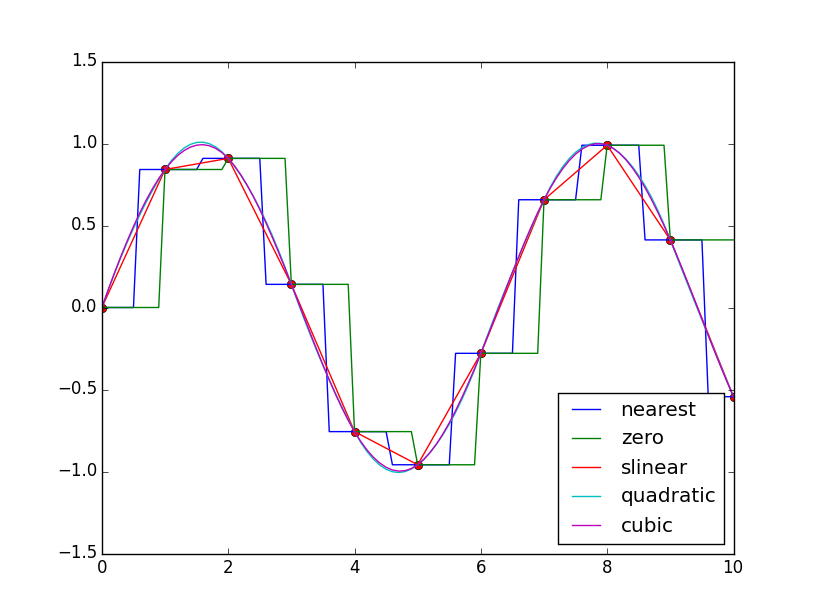

Two dimensional interpolation

The method is similar to one-dimensional data interpolation, which is two-dimensional spline interpolation.

# -*- coding: utf-8 -*-
"""
//Demonstrate 2D interpolation.
"""
import numpy as np
from scipy import interpolate
import pylab as pl
import matplotlib as mpl

def func(x, y):
    return (x+y)*np.exp(-5.0*(x**2 + y**2))

# The X-Y axis is divided into 15 * 15 grids
y,x= np.mgrid[-1:1:15j, -1:1:15j]

fvals = func(x,y) # Calculate the value of function 15 * 15 on each grid point
print len(fvals[0])

#Cubic spline 2D interpolation
newfunc = interpolate.interp2d(x, y, fvals, kind='cubic')

# Calculate the interpolation on the grid of 100 * 100
xnew = np.linspace(-1,1,100)#x
ynew = np.linspace(-1,1,100)#y
fnew = newfunc(xnew, ynew)#It's just a value of y value 100 * 100

# Mapping
# In order to compare the difference between before and after interpolation more clearly, the keyword parameter interpolation='nearest '
# Turn off the built-in interpolation operation of imshow().
pl.subplot(121)
im1=pl.imshow(fvals, extent=[-1,1,-1,1], cmap=mpl.cm.hot, interpolation='nearest', origin="lower")#pl.cm.jet
#Ext = [- 1,1, - 1,1] is x,y range favals is
pl.colorbar(im1)

pl.subplot(122)
im2=pl.imshow(fnew, extent=[-1,1,-1,1], cmap=mpl.cm.hot, interpolation='nearest', origin="lower")
pl.colorbar(im2)
pl.show()

• 1
• 2
• 3
• 4
• 5
• 6
• 7
• 8
• 9
• 10
• 11
• 12
• 13
• 14
• 15
• 16
• 17
• 18
• 19
• 20
• 21
• 22
• 23
• 24
• 25
• 26
• 27
• 28
• 29
• 30
• 31
• 32
• 33
• 34
• 35
• 36
• 37
• 38
• 39

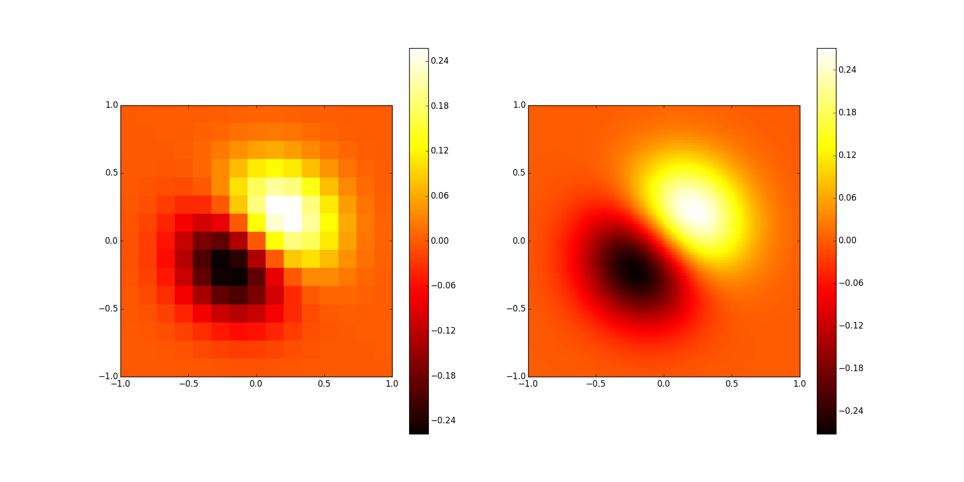
The left image is the original data, and the right image is the two-dimensional interpolation result.

3D display method of 2D interpolation

# -*- coding: utf-8 -*-
"""
//Demonstrate 2D interpolation.
"""
# -*- coding: utf-8 -*-
import numpy as np
from mpl_toolkits.mplot3d import Axes3D
import matplotlib as mpl
from scipy import interpolate
import matplotlib.cm as cm
import matplotlib.pyplot as plt

def func(x, y):
    return (x+y)*np.exp(-5.0*(x**2 + y**2))

# The X-Y axis is divided into 20 * 20 grids
x = np.linspace(-1, 1, 20)
y = np.linspace(-1,1,20)
x, y = np.meshgrid(x, y)#20 * 20 grid data

fvals = func(x,y) # Calculate the value of function 15 * 15 on each grid point

fig = plt.figure(figsize=(9, 6))
#Draw sub-graph1
ax=plt.subplot(1, 2, 1,projection = '3d')
surf = ax.plot_surface(x, y, fvals, rstride=2, cstride=2, cmap=cm.coolwarm,linewidth=0.5, antialiased=True)
ax.set_xlabel('x')
ax.set_ylabel('y')
ax.set_zlabel('f(x, y)')
plt.colorbar(surf, shrink=0.5, aspect=5)#Tagging

#Two dimensional interpolation
newfunc = interpolate.interp2d(x, y, fvals, kind='cubic')#newfunc is a function

# Calculate the interpolation on the grid of 100 * 100
xnew = np.linspace(-1,1,100)#x
ynew = np.linspace(-1,1,100)#y
fnew = newfunc(xnew, ynew)#Just the value of y value 100 * 100 np.shape(fnew) is 100*100
xnew, ynew = np.meshgrid(xnew, ynew)
ax2=plt.subplot(1, 2, 2,projection = '3d')
surf2 = ax2.plot_surface(xnew, ynew, fnew, rstride=2, cstride=2, cmap=cm.coolwarm,linewidth=0.5, antialiased=True)
ax2.set_xlabel('xnew')
ax2.set_ylabel('ynew')
ax2.set_zlabel('fnew(x, y)')
plt.colorbar(surf2, shrink=0.5, aspect=5)#Tagging

plt.show()

• 1
• 2
• 3
• 4
• 5
• 6
• 7
• 8
• 9
• 10
• 11
• 12
• 13
• 14
• 15
• 16
• 17
• 18
• 19
• 20
• 21
• 22
• 23
• 24
• 25
• 26
• 27
• 28
• 29
• 30
• 31
• 32
• 33
• 34
• 35
• 36
• 37
• 38
• 39
• 40
• 41
• 42
• 43
• 44
• 45
• 46
• 47
• 48

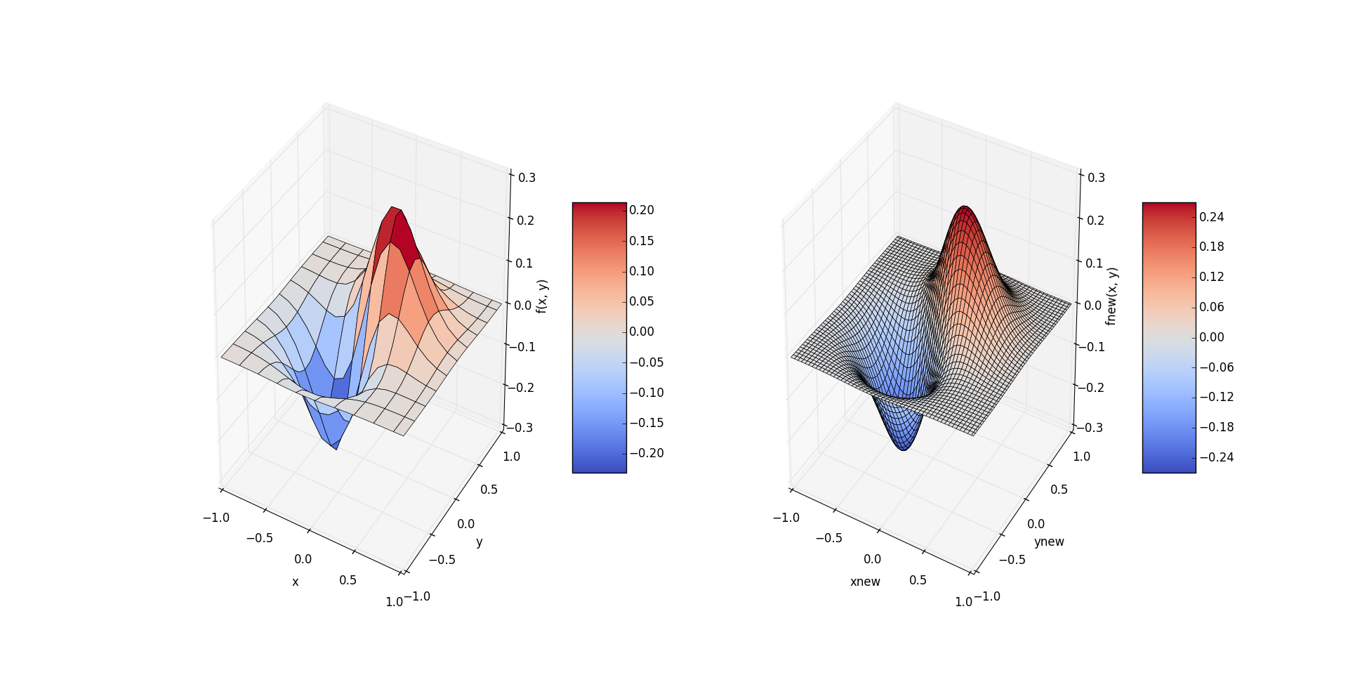
The function values of the two-dimensional data set in the left figure are rough because of the small number of samples. In the right figure, the sample values of more data points are obtained by cubic spline interpolation of the two-dimensional sample data, and the image is much smoother after drawing.