brief introduction

• Although logical regression bears the name of regression, it actually does classification. The general form of regression can be expressed as: f ( x ) = w x + b f(x)=wx+b f(x)=wx+b, however, the final result of the classification task is a determined label value, and the output range of the logistic regression is [- ∞, + ∞]. It is necessary to use the Sigmoid function to map the output Y to a probability value between [0,1], and then classify positive samples and negative samples according to the set threshold, such as > 0.5 as positive samples and < 0.5 as negative samples
• Logistic regression is called logarithmic probability function in Zhou Zhihua's watermelon book. In order to let the model predict derivatives approaching y, according to my understanding, it is extended from linear to nonlinear, so the logarithmic probability function can be expressed as: l n y = w x + b lny=wx+b lny=wx+b

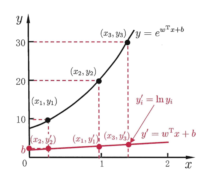
It can be seen from the figure that the logarithmic function here plays a role in connecting the predicted value of the linear regression model with the real marker [Zhou Zhihua, machine learning, p.56]

Sigmoid function

Sigmoid function is a mathematical function of S-shaped curve, which is widely used in logical regression and artificial neural network. The mathematical form of sigmoid function is:
S ( t ) = 1 1 + e − t S(t)=\frac{1}{1+e^{-t}} S(t)=1+e−t1​
The function image is as follows:

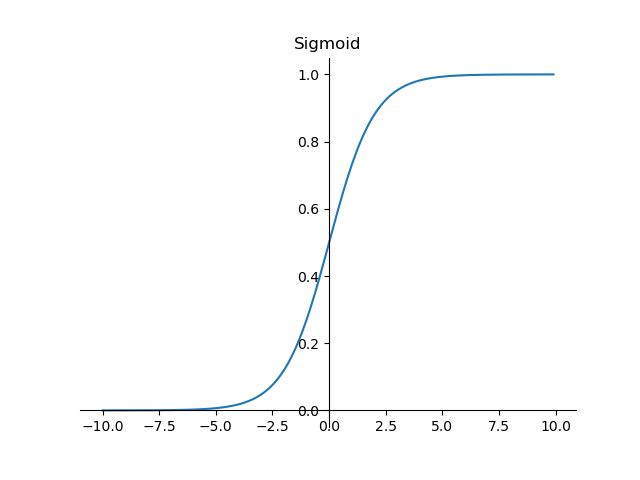
It can be seen that the sigmoid function is continuous, smooth, strictly monotonic, with (0,0.5) central symmetry, which is a very good threshold function.

In addition, sigmoid function has a very good feature. Its derivative function can be expressed by itself:
f ′ ( x ) = f ( x ) ( 1 − f ( x ) ) f'(x)=f(x)(1-f(x)) f′(x)=f(x)(1−f(x))

import matplotlib.pyplot as plt
import numpy as np

x = np.arange(-10,10,0.1)
y = 1/(1+np.exp(-x))


fig,ax = plt.subplots()
ax.plot(x,y)
ax.set_title('Sigmoid')
ax.spines['right'].set_color('none') # Hide the right border line
ax.spines['top'].set_color('none')    # Hide left border line
ax.xaxis.set_ticks_position('bottom')  # Set axis position
ax.yaxis.set_ticks_position('left')  # Set axis position
ax.spines['bottom'].set_position(('data', 0))   # Bind the coordinate axis position, and the data is determined by yourself according to the data
ax.spines['left'].set_position(('data', 0))
plt.show()

Loss function and parameter update

• w and b solution of general linear regression model

Linear regression tries to learn that f(x)=wx+b makes f(x) infinitely close to the value of Y. how to determine the value of W and B? The key is to measure the difference between f(x) and y. square loss, the mean square error, is usually used as a performance measure
( w ∗ , b ∗ ) = arg ⁡ min ⁡ ( w , b ) ∑ i = 1 m ( f ( x i ) − y i ) 2 = arg ⁡ min ⁡ ( w , b ) ∑ i = 1 m ( y i − w x i − b ) 2 \begin{aligned} \left(w^{*}, b^{*}\right) &=\underset{(w, b)}{\arg \min } \sum_{i=1}^{m}\left(f\left(x_{i}\right)-y_{i}\right)^{2} \\ &=\underset{(w, b)}{\arg \min } \sum_{i=1}^{m}\left(y_{i}-w x_{i}-b\right)^{2} \end{aligned} (w∗,b∗)​=(w,b)argmin​i=1∑m​(f(xi​)−yi​)2=(w,b)argmin​i=1∑m​(yi​−wxi​−b)2​
Solving w and b is to make E ( w , b ) = ∑ i = 1 m ( y i − w x i − b ) 2 E_{(w, b)}=\sum_{i=1}^{m}\left(y_{i}-w x_{i}-b\right)^{2} E(w,b) = Σ i=1m (yi − wxi − b)2 minimization process

• Solution of w and b in logistic regression

The probability loss function of logistic regression can be written as:
J ( θ ) = 1 2 m ∑ i = 1 m ( h θ ( x ( i ) ) − y ( i ) ) 2 = 1 2 m ∑ i = 1 m ( 1 1 + e − θ T x i − b − y ( i ) ) 2 J(\theta)=\frac{1}{2 m} \sum_{i=1}^{m}\left(h_{\theta}\left(x^{(i)}\right)-y^{(i)}\right)^{2}=\frac{1}{2 m} \sum_{i=1}^{m}\left(\frac{1}{1+e^{-\theta^{T} x_{i}-b}}-y^{(i)}\right)^{2} J(θ)=2m1​i=1∑m​(hθ​(x(i))−y(i))2=2m1​i=1∑m​(1+e−θTxi​−b1​−y(i))2
This loss function is nonconvex and difficult to optimize. It needs to be converted into maximum likelihood function to solve w and b

The probability of logistic regression can be integrated into:
p ( y ∣ x i ) = f ( x i ) y i ( 1 − f ( x i ) ) 1 − y i p(y|x_{i})=f(x_{i})^{y_{i}}(1-f(x_{i}))^{1-y_{i}} p(y∣xi​)=f(xi​)yi​(1−f(xi​))1−yi​
The likelihood function is:
L ( θ ) = ∏ i = 1 m P ( y i ∣ x i ; θ ) = ∏ i = 1 m ( h θ ( x i ) ) y i ( 1 − h θ ( x i ) ) 1 − y i L(\theta)=\prod_{i=1}^{m} P\left(y_{i} \mid x_{i} ; \theta\right)=\prod_{i=1}^{m}\left(h_{\theta}\left(x_{i}\right)\right)^{y_{i}}\left(1-h_{\theta}\left(x_{i}\right)\right)^{1-y_{i}} L(θ)=i=1∏m​P(yi​∣xi​;θ)=i=1∏m​(hθ​(xi​))yi​(1−hθ​(xi​))1−yi​
Log likelihood is:
l ( θ ) = log ⁡ L ( θ ) = ∑ i = 1 m ( y i log ⁡ h θ ( x i ) + ( 1 − y i ) log ⁡ ( 1 − h θ ( x i ) ) ) l(\theta)=\log L(\theta)=\sum_{i=1}^{m}\left(y_{i} \log h_{\theta}\left(x_{i}\right)+\left(1-y_{i}\right) \log \left(1-h_{\theta}\left(x_{i}\right)\right)\right) l(θ)=logL(θ)=i=1∑m​(yi​loghθ​(xi​)+(1−yi​)log(1−hθ​(xi​)))
Here, the gradient rise shall be used to find the maximum value and introduce J ( θ ) = − 1 m l ( θ ) J(\theta)=-\frac{1}{m}l(\theta) J( θ)= −m1​l( θ) Convert to gradient descent task

By deriving and simplifying the likelihood function:
δ δ θ j J ( θ ) = − 1 m ∑ i = 1 m ( y i 1 h θ ( x i ) δ δ θ j h θ ( x i ) − ( 1 − y i ) 1 1 − h θ ( x i ) δ δ θ j h θ ( x i ) ) \frac{\delta}{\delta_{\theta_{j}}} J(\theta)=-\frac{1}{m} \sum_{i=1}^{m}\left(y_{i} \frac{1}{h_{\theta}\left(x_{i}\right)} \frac{\delta}{\delta_{\theta_{j}}} h_{\theta}\left(x_{i}\right)-\left(1-\mathrm{y}_{\mathrm{i}}\right) \frac{1}{1-h_{\theta}\left(x_{i}\right)} \frac{\delta}{\delta_{\theta_{j}}} h_{\theta}\left(x_{i}\right)\right) δθj​​δ​J(θ)=−m1​i=1∑m​(yi​hθ​(xi​)1​δθj​​δ​hθ​(xi​)−(1−yi​)1−hθ​(xi​)1​δθj​​δ​hθ​(xi​))

= 1 m ∑ i = 1 m ( h θ ( x i ) − y i ) x i j =\frac{1}{m}\sum_{i=1}^{m}(h_{\theta}(x_{i})-y_{i})x_{i}^{j} =m1​i=1∑m​(hθ​(xi​)−yi​)xij​

Softmax

https://zhuanlan.zhihu.com/p/105722023

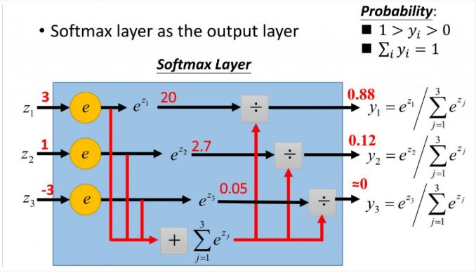
Compared with softmax, hardmax means that only one of the maximum values is selected. Softmax means that it no longer uniquely determines a maximum value, but assigns a probability value to each output classification result, indicating the possibility of belonging to each category.

Definition of softmax function:
Softmax ⁡ ( z i ) = e z i ∑ c = 1 C e z c \operatorname{Softmax}\left(z_{i}\right)=\frac{e^{z_{i}}}{\sum_{c=1}^{C} e^{z_{c}}} Softmax(zi​)=∑c=1C​ezc​ezi​​
Where, Zi is the output value of the ith node, and C is the number of output nodes, that is, the number of categories classified.

Why use the softmax function?

• The output value can be separated

Experiment with the code. Suppose there are three output node values (1, 5, 10, 15)

import numpy as np
x = np.array([1,5,10,15])
y = np.exp(x) #  array([2.71828183e+00, 1.48413159e+02, 2.20264658e+04, 3.26901737e+06])
S = np.exp(x)/sum(y) # array([8.25925493e-07, 4.50940040e-05, 6.69254359e-03, 9.93261536e-01])
# Let's find the solution without exponential form
Z = x/sum(x) #  array([0.03225806, 0.16129032, 0.32258065, 0.48387097])

The result is obvious, using the exponential form to pull the value with large gap even larger

• The second advantage is that the derivative of ex is still ex

For the derivation process, please refer to the following two Blogs: https://www.jianshu.com/p/4670c174eb0d https://www.jianshu.com/p/6e405cecd609

The result after derivation can be expressed as:
∂ L i ∂ W i j = { ( S i − 1 ) x j , y = i S i x j , y ≠ i ∂ L i ∂ b i = { ( S i − 1 ) , y = i S i , y ≠ i \begin{aligned} &\frac{\partial L_{i}}{\partial W_{i j}}= \begin{cases}\left(S_{i}-1\right) x_{j} & , y=i \\ S_{i} x_{j} & , y \neq i\end{cases} \\ &\frac{\partial L_{i}}{\partial b_{i}}= \begin{cases}\left(S_{i}-1\right) & , y=i \\ S_{i} & , y \neq i\end{cases} \end{aligned} ​∂Wij​∂Li​​={(Si​−1)xj​Si​xj​​,y=i,y​=i​∂bi​∂Li​​={(Si​−1)Si​​,y=i,y​=i​​
Where S is the softmax function and y is the tag value. Corresponding code:

def L_Gra(W, b, x, y):
    """
     W,b For the current weight and offset parameters, x，y It is the sample data and the label corresponding to the sample
    """
    # initialization
    W_G = np.zeros(W.shape)
    b_G = np.zeros(b.shape)
    S = softmax(np.dot(W,x) + b)
    W_row = W.shape[0]
    W_column = W.shape[1]
    b_column = b.shape[0]

    # Find the gradient for Wij and bi respectively
    for i in range(W_row):
        for j in range(W_column):
            W_G[i][j] = (S[i] - 1) * x[j] if y == i else S[i] * x[j] # S: Why is loss not used in the softmax function? It has been added in the solution process

    for i in range(b_column):
        b_G[i] = S[i] - 1 if y == i else S[i]
    return W_G, b_G

def L_Gra(W, b, x, y):
    """
     W, b For the current weight and offset parameters, x,y It is the sample data and the label corresponding to the sample
    """
    #initialization
    W_G = np.zeros(W.shape)
    b_G = np.zeros(b.shape)
    S = softmax(np.dot(W,x) + b)
    W_row=W.shape[0]
    W_column=W.shape[1]
    b_column=b.shape[0]
    #Find the gradient for Wij and bi respectively
    for i in range(W_row):
        for j in range(W_column):
            W_G[i][j]=(S[i] - 1) * x[j] if y==i else S[i]*x[j]
               
    for i in range(b_column):
        b_G[i]=S[i]-1 if y==i else S[i]
    #Returns the gradient of W and b    
    return W_G, b_G

The complete code is as follows

#!/usr/bin/env python
# -*- coding:utf-8 -*-
# @FileName  :lr_mnist.py
# @Time      :2021/10/22 14:44
# @Author    :nin
import time

import numpy as np
import pandas as pd
import gzip as gz
import matplotlib.pyplot as plt
from tqdm import tqdm
from tqdm import trange
# ------------Read data-------------- #
# filename is the file name, kind is' data 'or' label '
def load_data(filename,kind):
    with gz.open(filename, 'rb') as fo:  # Open the compressed file using the gzip module
        buf = fo.read()                 # Read the compressed content into the cache. b '' indicates that this is a bytes object
        index = 0
        if kind == 'data':
            # Because the data types of the first four rows in the data structure are 32-bit integers, the i format is adopted, and the first four rows of data need to be read, so four i's are required
            header = np.frombuffer(buf, '>i', 4, index)
            index += header.size * header.itemsize
            data = np.frombuffer(buf, '>B', header[1] * header[2] * header[3], index).reshape(header[1], -1) # 2-d matrix
        elif kind == 'lable':
            # Because the data types of the first two rows in the data structure are 32-bit integers, the i format is adopted, and the first two rows of data need to be read, so two i's are required
            header = np.frombuffer(buf, '>i', 2, 0)
            index += header.size * header.itemsize
            data = np.frombuffer(buf,'>B', header[1], index)
    return data

# -----------Load data------------- #
X_train = load_data('train-images-idx3-ubyte.gz','data')
y_train = load_data('train-labels-idx1-ubyte.gz','lable')
X_test = load_data('t10k-images-idx3-ubyte.gz','data')
y_test = load_data('t10k-labels-idx1-ubyte.gz','lable')
# -----------View data format------------- #
print('Train data shape:')
print(X_train.shape, y_train.shape)
print('Test data shape:')
print(X_test.shape, y_test.shape)

"""# -----------Data visualization------------- #
index_1 = 1024
plt.imshow(np.reshape(X_train[index_1], (28,28)), cmap='gray')
plt.title('Index:{}'.format(index_1))
plt.show()
print("Label: {}".format(y_train[index_1]))

index_2 = 2048
plt.imshow(np.reshape(X_train[index_2], (28,28)), cmap='gray')
plt.title('Index:{}'.format(index_2))
plt.show()
print('Label: {}'.format(y_train[index_2]))"""

# -----------Define constants------------- #
x_dim = 28 * 28  # data shape, 28*28
y_dim = 10      # output shape, 10*1
W_dim = (y_dim, x_dim)  # Matrix W
b_dim = y_dim    # index b
# -----------definition logistic regression Necessary functions in------------- #
# Softmax function
def softmax(x):
    """
    :param x:
    :return: through softmax Transformed vector
    """
    return np.exp(x) / np.exp(x).sum()

# Loss function
# L = -log(Si(yi)), yi is the predicted value
def loss(W,b,x,y):
    """
    W, b For the current weight and offset parameters, x，y It is the sample data and the label corresponding to the sample
    """
    return -np.log(softmax(np.dot(W,x) + b)[y]) # The probability that the predicted value is the same as the label

# Single sample loss function gradient
def L_Gra(W, b, x, y):
    """
     W,b For the current weight and offset parameters, x，y It is the sample data and the label corresponding to the sample
    """
    # initialization
    W_G = np.zeros(W.shape)
    b_G = np.zeros(b.shape)
    S = softmax(np.dot(W,x) + b)
    W_row = W.shape[0]
    W_column = W.shape[1]
    b_column = b.shape[0]

    # Find the gradient for Wij and bi respectively
    for i in range(W_row):
        for j in range(W_column):
            W_G[i][j] = (S[i] - 1) * x[j] if y == i else S[i] * x[j] # S: Why is loss not used in the softmax function? It has been added in the solution process

    for i in range(b_column):
        b_G[i] = S[i] - 1 if y == i else S[i]
    return W_G, b_G

# Verify the correctness of the model on the test set
def test_accurate(W, b, X_test, y_test):
    num = len(X_test)
    # Save the test results in results. Add a 1 if it is correct and a 0 if it is wrong
    results = []
    for i in range(num):
        # Check whether the subscript of the largest element in softmax(W*x+b) is y. if so, the prediction is correct
        y_i = np.dot(W,X_test[i]) + b   # X_test is equivalent to 784 characteristic points, W is the weight matrix and y_i is the predicted value
        res = 1 if softmax(y_i).argmax() == y_test[i] else 0    # Compare with the real label value to judge whether the prediction is correct
        results.append(res)

    accurate_rate = np.mean(results)
    return accurate_rate

# ------------------- #
# Gradient descent method
# ------------------- #
def mini_batch(batch_size, lr, epoches):
    """
    batch_size by batch The size of the, lr Is the step size, epoches by epoch Number of training sessions
    """
    accurate_rates = []     # Record the correct rate of each iteration
    iters_W = []    # Record the W for each iteration
    iters_b = []    # Record b for each iteration

    W = np.zeros(W_dim)
    b = np.zeros(b_dim)
    # Batch the original samples and labels according to the size of batch_size
    # initialization
    x_batches = np.zeros(((int(X_train.shape[0]/batch_size), batch_size, 784)))
    y_batches = np.zeros(((int(X_train.shape[0]/batch_size), batch_size)))
    batch_num = int(X_train.shape[0]/batch_size)
    # in batches
    for i in range(0, X_train.shape[0], batch_size):
        x_batches[int(i/batch_size)] = X_train[i:i + batch_size]
        y_batches[int(i/batch_size)] = y_train[i:i + batch_size]
    print('Start training...')

    for epoch in range(epoches):
        print("epoch:{}".format(epoch))
        start = time.time()
        with trange(batch_num) as t:
          for i in t:    # i is batch
            # Set the information displayed on the left of the progress bar
            t.set_description("epoch %i" % epoch)
            # Set the information displayed on the right side of the progress bar
            # t.set_postfix(loss=random(), gen=randint(1, 999), str="h", lst=[1, 2])
            # init grads
            W_gradients = np.zeros(W_dim)      # (10,784)
            b_gradients = np.zeros(b_dim)      # (10,1)

            x_batch, y_batch = x_batches[i], y_batches[i]
            # j is a single sample
            for j in range(batch_size): # The lower gradient value is calculated for each sample in each batch
                W_g, b_g = L_Gra(W, b, x_batch[j], y_batch[j])   # Calculate the gradient value of a single sample
                W_gradients += W_g  # Gradient accumulation
                b_gradients += b_g
            W_gradients /= batch_size   # Accumulated / m is the batch size
            b_gradients /= batch_size
            # Gradient descent
            W -= lr * W_gradients
            b -= lr * b_gradients
            # Record the values of total W and b after each iteration
            iters_W.append(W.copy())
            iters_b.append(b.copy())

        # epoch runs one test at the end of each run
        end = time.time()
        time_cost = (end - start)
        print("time cost:{}s".format(time_cost))
        accurate_rates.append(test_accurate(W, b, X_test, y_test))

    return W, b, time_cost, accurate_rates, iters_W, iters_b

def run(lr, batch_size, epochs_num):
    """
    W ,b : w and b Optimal solution of
    W_s, b_s : Value obtained after each iteration
    """
    W, b, time_cost, accuracys, W_s, b_s = mini_batch(batch_size, lr, epochs_num)
    # Find the distance between W and b and the optimal solution, and use the second-order norm to express the distance
    iterations = len(W_s)
    dis_W = []
    dis_b = []

    for i in range(iterations):
        # Calculate the Euclidean distance between each iteration and the final W
        dis_W.append(np.linalg.norm(W_s[i] - W))
        dis_b.append(np.linalg.norm(b_s[i] - b))

    print("the parameters is: step length alpah:{}; batch size:{}; Epoches:{}".format(lr, batch_size, epochs_num))
    print("Result: accuracy:{:.2%},time cost:{:.2f}".format(accuracys[-1], time_cost))
    # ----------------Mapping-------------- #
    # Variation of accuracy with number of iterations
    plt.title('The Model accuracy variation chart ')
    plt.xlabel('Iterations')
    plt.ylabel('Accuracy')
    plt.plot(accuracys,'m')
    plt.grid()
    plt.show()
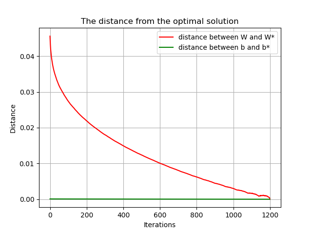
    # The distance between W and b and the optimal solution varies with the number of iterations
    plt.title('The distance from the optimal solution')
    plt.xlabel('Iterations')
    plt.ylabel('Distance')
    plt.plot(dis_W, 'r', label='distance between W and W*')
    plt.plot(dis_b, 'g', label='distance between b and b*')
    plt.legend()
    plt.grid()
    plt.show()

# ----------Parameter input---------------
lr = 1e-5
batch_size = 10000
epochs_num = 20
# Run function
run(lr, batch_size, epochs_num)

lr = 1e-5 bs = 1000 epoch=20