1, ndarray object
1. Install Numpy: on the command line, enter pip install numpy
2.ndarray object -- a core data structure around Numpy
The ndarray object is an N-dimensional array. But note that ndarray is homogeneous. Homogeneity means that all elements in an N-dimensional array must belong to the same data type. PS: list s in Python are heterogeneous.
After the ndarray object is instantiated, it contains some basic properties.
- Shape: the shape of the ndarray object, represented by a tuple;
- Ndim: Dimension of ndarray object;
- Size: number of elements in the ndarray object;
- Dtype: the data type of the element in the ndarray object, such as int64, float32, etc
# Import numpy and alias it np
import numpy as np
# Construct ndarray
a = np.arange(15).reshape(3,5)
#   The shape of ndarray is (3, 5) (representing 3 rows and 5 columns);
#   ndim is 2 (because the matrix has two dimensions: row and column);
#   size is 15 (because the matrix has a total of 15 elements);
#   dtype is int32 (because the elements in the matrix are integers and 32-bit integers are enough to represent the elements in the matrix)
print(a.shape)
print(a.ndim)
print(a.size)
print(a.dtype)
3. Instantiate the ndarray object
import numpy as np
# Instantiate the ndarray object a using the list as the initial value
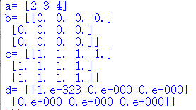
a = np.array([2,3,4])
print("a=",a)
# Instantiate the ndarray object b, which is a matrix with 3 rows and 4 columns. All elements in the matrix are 0
b = np.zeros((3, 4))
print("b=",b)
# Instantiate the ndarray Object c, which is a matrix with 3 rows and 4 columns. All elements in the matrix are 1
c = np.ones((3, 4))
print("c=",c)
# Instantiate the ndarray object d, which is a matrix with 2 rows and 3 columns. All elements in the matrix are random values
d = np.empty((2, 3))
print("d=",d)
First pass
import numpy as np


def print_ndarray(input_data):
    '''
    instantiation  ndarray Object and print
    :param input_data: Test case, dictionary type
    :return: None
    '''

    #********* Begin *********#
    a = np.array(input_data['data'])
    print(a)
    #********* End *********#
2, Shape operation
Change the shape of the ndarray object:
import numpy as np
a = np.zeros((3, 4))

# Modify shape properties directly (too rough, not in line with good programming practices)
a.shape = [4, 3]
print(a)


# Call the member function reshape of a to change 3 rows and 4 columns into 4 rows and 3 columns
a = a.reshape((4, 3))   #Object oriented bias
print(a)
# Call the reshape function to change a into 4 rows and 3 columns
a = np.reshape(a, (4, 3))   #Biased process oriented
print(a)
#   PS: no matter which method of reshape is used, the shape of the original ndarray will not be changed. Instead, the source ndarray will be deeply copied and deformed, and finally the deformed array will be returned.
#   That is, if the code is np.reshape(a, (4, 3)), the shape of a will not be modified!


# Change a from a two-dimensional array with 3 rows and 4 columns to a one-dimensional array with 12 elements
a.resize(12)    #Directly change the shape of the source ndarray
print(a)


#During deformation, if the value in a dimension is - 1, the value in that dimension will be automatically calculated according to the values in other dimensions.
# Filling - 1 in the dimension of rows will allow numpy to calculate the number of trips. Obviously, the number of rows should be 24
a = a.reshape((-1, 2))
print(a)
#If the code is changed to a = a.reshape((-1, -1)), NumPy will throw an exception ValueError: can only specify one unknown dimension.
Second pass
import numpy as np


def reshape_ndarray(input_data):
    '''
    take ipnut_data convert to ndarray Then it is changed into a bit array and printed
    :param input_data: Test case of type list
    :return: None
    '''

    #********* Begin *********#
    a = np.array(input_data)
    a = a.reshape((1,-1))
    print(a[0,])
    #********* End *********#
3, Basic operation
Arithmetic operation:
If you want to do elementwise arithmetic operations on the elements in the ndarray object, it is very simple. Add, subtract, multiply and divide.
import numpy as np

a = np.array([0, 1, 2, 3])

b = a + 2    # Add 2 to all elements in a and the result is [2, 3, 4, 5]

c = a - 2    # All elements in a are subtracted by 2, and the result is [- 2, - 1, 0, 1]

d = a * 2    # All elements in a are multiplied by 2 and the result is [0, 2, 4, 6]

e = a ** 2    # All elements in a are squared and the result is [0, 1, 4, 9]

f = a / 2    # All elements in a are divided by 2 and the result is [0, 0.5, 1, 1.5]

g = a < 2    # All elements in a are compared with 2, and the result is [True, True, False, False]
Matrix operation:
The elementwise operation between matrix A and matrix B of the same shape is also very simple. Add, subtract, multiply and divide.
import numpy as np
a = np.array([[0, 1], [2, 3]])
b = np.array([[1, 1], [3, 2]])

c = a + b   # a and b are added one by one, and the result is [[1,2], [5,5]]

d = a - b    # a and b are subtracted one by one, and the result is [[- 1, 0], [- 1, 1]]

e = a * b    # a and b are multiplied element by element, and the result is [[0,1], [6,6]]

f = a / b    # Divide element by element of a by element of b, and the result is [[0,1.], [0.6667,1.5]]

g = a ** b    # a and b perform power operation one by one, and the results are [[0, 1], [8, 9]]

h = a < b    # Comparing a and b element by element, the result is [[True, False], [True, False]]

#   *Can only do elementwise operation. If you want to do real matrix multiplication, you obviously can't use *.
#   NumPy provides @ and dot functions to implement matrix multiplication.
A = np.array([[1, 1], [0, 1]])
B = np.array([[2, 0], [3, 4]])

print(A @ B)    # @Represents matrix multiplication, matrix A is multiplied by matrix B, and the result is [[5,4], [3,4]]

print(A.dot(B)) # In object-oriented style, matrix A is multiplied by matrix B, and the result is [[5,4], [3,4]]

print(np.dot(A, B)) # For process style, matrix A is multiplied by matrix B, and the result is [[5,4], [3,4]]
Simple statistics:
import numpy as np
a = np.array([[-1, 1, 2, 3], [4, 5, 6, 7], [8, 9, 10, 13]])
print(a.sum())   # Calculate the sum of all elements in a and the result is 67

print(a.max())    # Find the largest element in a and the result is 13

print(a.min())    # Find the smallest element in a and the result is - 1

print(a.argmax())    # Find out the position of the largest element in A. since there are 12 elements in a, the position starts from 0, so the result is 11

print(a.argmin())    # Find the position of the smallest element in a, and the result is 0
The dimension is 2, which means that there are two axes: axis 0 and axis 1 (the number of axes starts from 0).
Axis 0 is the vertical axis and axis 1 is the horizontal axis. To realize the statistics along which axis, you only need to modify axis
When axis is not modified, the default value of axis is None, which means that all elements in the ndarray object will be taken into account in statistics.
    import numpy as np
    info = np.array([[3000, 4000, 20000], [2700, 5500, 25000], [2800, 3000, 15000]])

   	print(info.min(axis=0)) 	# According to the statistics along axis 0, the result is [2700, 3000, 15000]

    print(info.max(axis=0)) 	# According to the statistics along axis 0, the result is [3000, 5500, 25000]
Third pass
import numpy as np


def get_answer(input_data):
    '''
    take input_data convert to ndarray Count the position of the maximum value in each line and print it
    :param input_data: Test case of type list
    :return: None
    '''

    #********* Begin *********#
    a = np.array(input_data)
    print(a.argmax(axis=1))
    #********* End *********#
4, Random number generation
Simple random number generation
Random_sample: random_sample is used to generate random numbers with an interval of [0,1]. The parameter size to be filled in indicates the shape of the generated random number. For example, if size = [2,3], a 2-row and 3-column ndarray will be generated and filled with random values.
Choice: a random value is a discrete value and can be implemented using choice if the range is known.
The main parameters of choice are a, size and replace. A is a one-dimensional array, which means you want to randomly select from a; size is the shape after the random number is generated. If you simulate 5 dice rolls, replace is used to set whether the same elements can be taken. True means the same number can be taken; False means the same number cannot be taken. The default is true.
randint: randint has the same function as choice, but randint can only generate integers, and the number generated by choice is related to A. if there are floating-point numbers in a, choice will have the probability to select floating-point numbers.
randint has three parameters: low, high and size. Where low represents the minimum value that can be generated when generating random numbers, and high represents the maximum value that can be generated when generating random numbers minus 1. That is to say, the interval of random numbers generated by randint is [low, high].
import numpy as np

'''
The result may be[[0.32343809, 0.38736262, 0.42413616]
          [0.86190206, 0.27183736, 0.12824812]]
'''
print(np.random.random_sample(size=[2, 3]))


'''
The number of points that may occur when rolling dice is 1, 2, 3, 4, 5, 6,therefore a=[1,2,3,4,5,6]
Simulate 5 this dice roll, so size=5
 The result may be [1 4 2 3 6]
'''
print(np.random.choice(a=[1, 2, 3, 4, 5, 6], size=5,replace=False))


'''
The number of points that may occur when rolling dice is 1, 2, 3, 4, 5, 6,therefore low=1,high=7
 Simulate 5 this dice roll, so size=5
 The result may be [6, 4, 3, 1, 3]
'''
print(np.random.randint(low=1, high=7, size=5))
Probability distribution random number generation
Gaussian distribution, also known as normal distribution, is high in the middle and low on both sides. The horizontal axis represents the value of the random variable (which can be regarded as the generated random value), and the vertical axis represents the corresponding probability of the random variable (which can be regarded as the probability that the random value is selected).
Normal: in addition to the size parameter, two more important parameters of normal function are loc and scale, which represent the mean and variance of Gaussian distribution respectively. The position of the point with the highest probability in the distribution affected by loc. Assuming loc=2, the position of the point with the highest probability in the distribution is 2. Scale affects the weight of the distribution graph. The smaller the scale, the higher and thinner the distribution. The larger the scale, the shorter and fatter the distribution.
import numpy as np
'''
Generate 5 random numbers according to Gaussian distribution
 The results may be:[1.2315868, 0.45479902, 0.24923969, 0.42976352, -0.68786445]
It can be seen from the results that 0.4 The left and right values appear more frequently, 1 and-0.7 The number of occurrences of the left and right values is relatively low.
'''
print(np.random.normal(size=5))


#Five random values are generated according to the Gaussian distribution with mean value of 1 and variance of 10
print(np.random.normal(loc=1, scale=10, size=5))
Random seed
The random number generated by the computer is the value calculated by the random seed according to a certain calculation method. So as long as the calculation method is fixed and the random seed is fixed, the generated random number will not change!
If you want to keep the random number generated each time unchanged, you need to set the random seed (the random seed is actually an integer from 0 to 232 − 1). Setting the random seed is very long and simple. Just call the seed function and set the random seed.
    import numpy as np
    # Set random seed to 233
    np.random.seed(seed=233)
    data = [1, 2, 3, 4]
    # Randomly select the number from the data, and the result is 4
    print(np.random.choice(data))
    # Randomly select the number from the data, and the result is 4
    print(np.random.choice(data))
The fourth level
import numpy as np


def shuffle(input_data):
    '''
    Upset input_data And return the disruption result
    :param input_data: Test case input, type list
    :return: result,Type is list
    '''

    # Save scrambled results
    result = []
    #********* Begin *********#
    result = list(np.random.choice(a=input_data,size=len(input_data),replace=False))
    #********* End *********#
    return result
5, Indexing and slicing
Indexes:
The index of ndarray is actually very similar to the index of python's list. The index of the element starts at 0.
    import numpy as np
    # If there are 4 elements in a, the indexes of these elements are 0, 1, 2 and 3 respectively
    a = np.array([2, 15, 3, 7])
    # Print the second element. Index 1 represents the second element in a, and the result is 15
    print(a[1])
    # b is a two-dimensional array with 2 rows and 3 columns
    b = np.array([[1, 2, 3], [4, 5, 6]])
    # Print the first line in b, there are two lines in total, so the indexes of the lines are 0 and 1 respectively, and the result is [1, 2, 3]
    print(b[0])
    # Print the elements in Row 2 and column 2 in b, and the result is 5
    print(b[1][1])
Traversal:
The traversal of ndarray is also very similar to that of python's list
    import numpy as np
    a = np.array([2, 15, 3, 7])
    # Use the for loop to take out the elements in a and print them
    for element in a:
        print(element)
    # Traverse the elements in a according to the index and print
    for idx in range(len(a)):
        print(a[idx])
    # b is a two-dimensional array with 2 rows and 3 columns
    b = np.array([[1, 2, 3], [4, 5, 6]])
    # Expand b into a one-dimensional array, traverse and print
    for element in b.flat:
        print(element)
    # Traverse the elements in b according to the index and print
    for i in range(len(b)):
        for j in range(len(b[0])):
            print(b[i][j])
section:
The slicing method of ndarray is also very similar to the traversal method of python's list.
When slicing, the index range is closed left and open right.
import numpy as np
# If there are 4 elements in a, the indexes of these elements are 0, 1, 2 and 3 respectively
a = np.array([2, 15, 3, 7])

'''
Slice out and print all elements of the index from 1 to the end
 The result is[15  3  7]
'''
print(a[1:])


'''
Slice out and print all elements from the penultimate to the last
 The result is[3  7]
'''
print(a[-2:])


'''
Slice and print all elements in reverse order
 The result is[ 7  3 15  2]
'''
print(a[::-1])


# b is a two-dimensional array with 2 rows and 3 columns
b = np.array([[1, 2, 3], [4, 5, 6]])

'''
Slice and print all elements from column 2 to column 3 of row 2
 The result is[[5 6]]
'''
print(b[1:, 1:3])


'''
Slice and print all elements from columns 2 to 3
 The result is[[2 3]
    [5 6]]
'''
print(b[:, 1:3])
Fifth pass
import numpy as np

def get_roi(data, x, y, w, h):
    '''
    extract data The vertex coordinates of the upper left corner of the middle are(x, y)Width is w Gao Wei h of ROI
    :param data: Two dimensional array of type ndarray
    :param x: ROI The row index of the top left vertex of type int
    :param y: ROI The column index of the top left vertex of type int
    :param w: ROI Width of, type int
    :param h: ROI High, type int
    :return: ROI,Type is ndarray
    '''

    #********* Begin *********#
    a = data[x:x+h+1,y:y+w+1]
    return a
    #********* End *********#