NO.89 - Applying Xgboost to Predict Insurance Compensation

Article Directory

1 Data analysis
1.1 First look at what the data looks like
1.2 Continuous and categorical variables
1.3 Number of attributes in categorical variables
1.4 Compensation value
1.5 Continuous Variable Characteristics
1.6 Correlation between features
2 Xgboost
2.1 Data Preprocessing
2.2 Simple Xgboost model
2.3 First Base Model
2.4 Xgboost Parameter Adjustment
3 Summary

1 Data analysis

import pandas as pd
import numpy as np
import matplotlib.pyplot as plt
from sklearn.linear_model import LogisticRegression
from sklearn.ensemble import RandomForestClassifier
from sklearn.metrics import roc_auc_score as AUC
from sklearn.metrics import mean_absolute_error
from sklearn.decomposition import PCA
from sklearn.preprocessing import LabelEncoder, LabelBinarizer
from sklearn.model_selection import cross_val_score

from scipy import stats
import seaborn as sns
from copy import deepcopy

%matplotlib inline

# This may raise an exception in earlier versions of Jupyter
%config InlineBackend.figure_format = 'retina'

1.1 First look at what the data looks like

train = pd.read_csv('train.csv')
test = pd.read_csv('test.csv')
train.shape

(188318, 132)

print ('First 20 columns:', list(train.columns[:20]))

print ('Last 20 columns:', list(train.columns[-20:]))

First 20 columns: ['id', 'cat1', 'cat2', 'cat3', 'cat4', 'cat5', 'cat6', 'cat7', 'cat8', 'cat9', 'cat10', 'cat11', 'cat12', 'cat13', 'cat14', 'cat15', 'cat16', 'cat17', 'cat18', 'cat19']
Last 20 columns: ['cat112', 'cat113', 'cat114', 'cat115', 'cat116', 'cont1', 'cont2', 'cont3', 'cont4', 'cont5', 'cont6', 'cont7', 'cont8', 'cont9', 'cont10', 'cont11', 'cont12', 'cont13', 'cont14', 'loss']

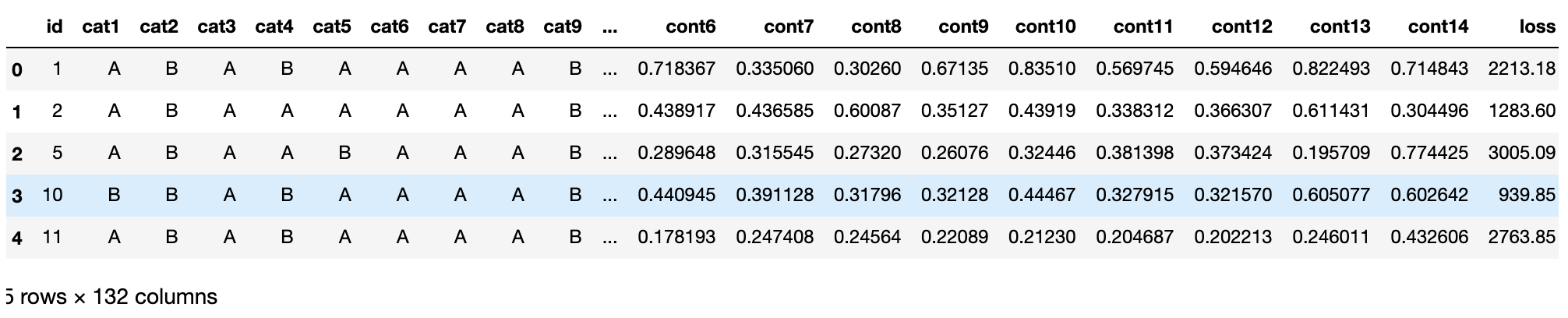
We can see that there are approximately 116 species attributes (as their names show) and 14 consecutive (numeric) attributes.In addition, there are ID s and compensation.The total is 132 columns.

train.head(5)

train.describe()

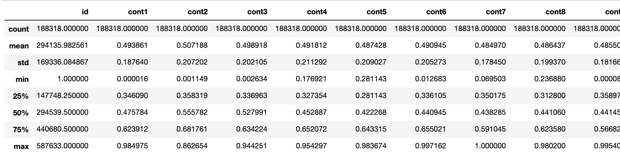
As we can see, all continuous functions have been scaled to [0,1] intervals, with a mean of almost 0.5.Actually, the data has already been preprocessed. What we get is the feature data.

View missing values

pd.isnull(train).values.any()

False

1.2 Continuous and categorical variables

train.info()

<class 'pandas.core.frame.DataFrame'>
RangeIndex: 188318 entries, 0 to 188317
Columns: 132 entries, id to loss
dtypes: float64(15), int64(1), object(116)
memory usage: 189.7+ MB
Here, float64(15) is the 14 continuous variable + loss value; int64(1) is the ID;
object(116) is a classification variable.

cat_features = list(train.select_dtypes(include=['object']).columns)
print ("Categorical: {} features".format(len(cat_features)))

Categorical: 116 features

cont_features = [cont for cont in list(train.select_dtypes(
                 include=['float64', 'int64']).columns) if cont not in ['loss', 'id']]
print ("Continuous: {} features".format(len(cont_features)))

Continuous: 14 features

id_col = list(train.select_dtypes(include=['int64']).columns)
print ("A column of int64: {}".format(id_col))

A column of int64: ['id']

1.3 Number of attributes in categorical variables

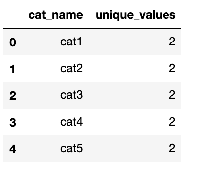
cat_uniques = []
for cat in cat_features:
    cat_uniques.append(len(train[cat].unique()))
    
uniq_values_in_categories = pd.DataFrame.from_items([('cat_name', cat_features), ('unique_values', cat_uniques)])

uniq_values_in_categories.head()

1.4 Compensation value

plt.figure(figsize=(16,8))
plt.plot(train['id'], train['loss'])
plt.title('Loss values per id')
plt.xlabel('id')
plt.ylabel('loss')
plt.legend()
plt.show()

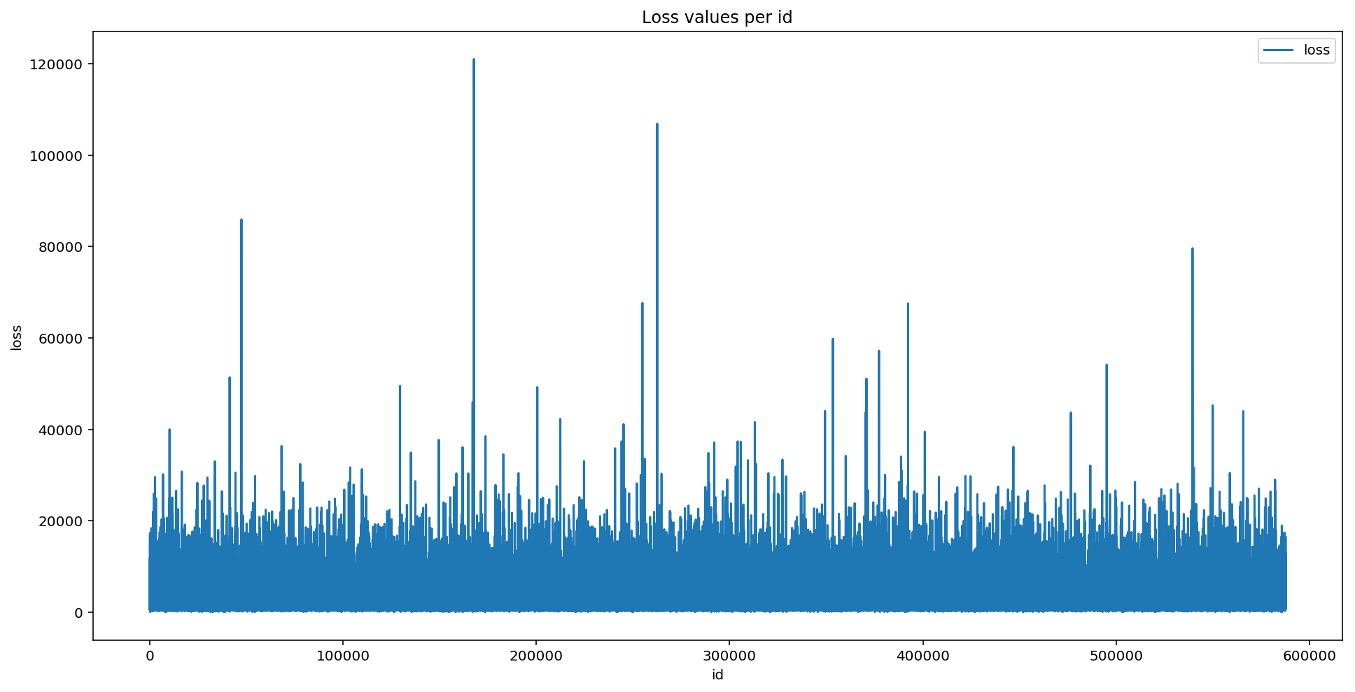
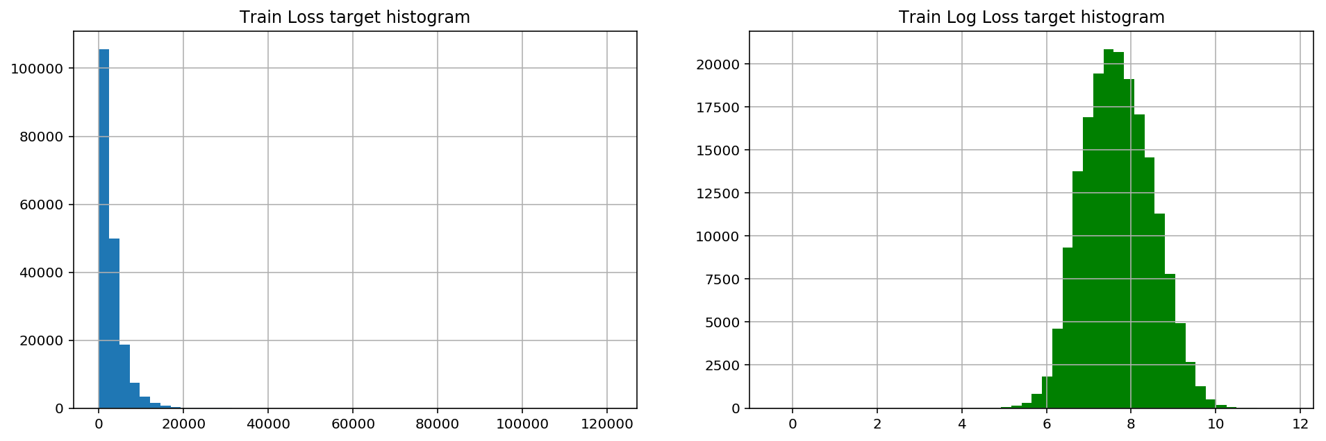
Several significant peaks in the loss values represent serious accidents.This distribution of data makes regression performance poor due to very distorted functionality.

Basically, skewness measures the asymmetry of the mean distribution of real random variables.Let's calculate the skewness of the loss:

stats.mstats.skew(train['loss']).data

array(3.79492815)

A skewness greater than 1 indicates that the data is indeed skewed

Logarithmic transformation of the data usually improves skewing, using np.log

stats.mstats.skew(np.log(train['loss'])).data

array(0.0929738)

fig, (ax1, ax2) = plt.subplots(1,2)
fig.set_size_inches(16,5)
ax1.hist(train['loss'], bins=50)
ax1.set_title('Train Loss target histogram')
ax1.grid(True)
ax2.hist(np.log(train['loss']), bins=50, color='g')
ax2.set_title('Train Log Loss target histogram')
ax2.grid(True)
plt.show()

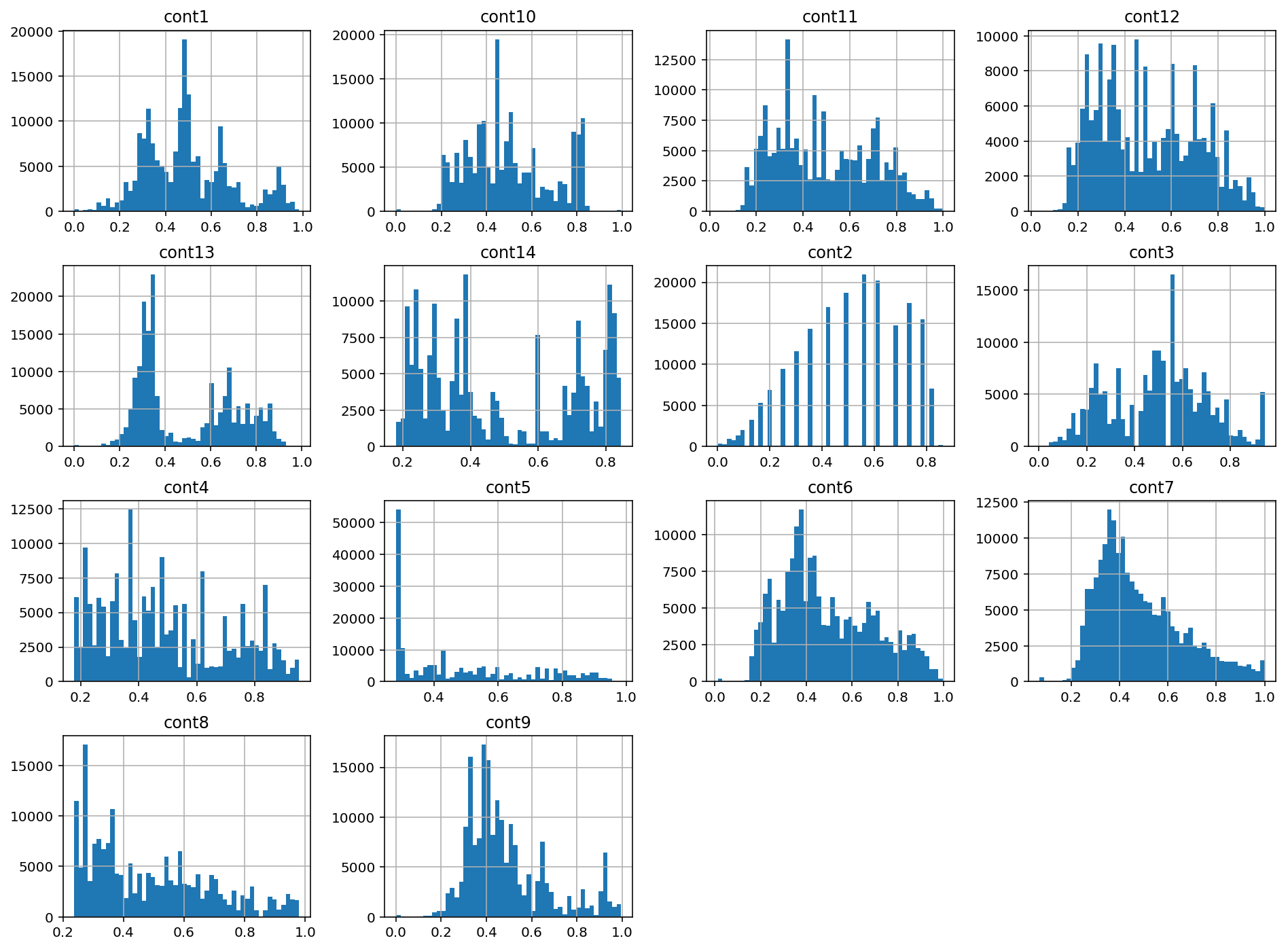
1.5 Continuous Variable Characteristics

train[cont_features].hist(bins=50, figsize=(16,12))

1.6 Correlation between features

plt.subplots(figsize=(16,9))
correlation_mat = train[cont_features].corr()
sns.heatmap(correlation_mat, annot=True)

2 Xgboost

import xgboost as xgb
import pandas as pd
import numpy as np
import pickle
import sys
import matplotlib.pyplot as plt
from sklearn.metrics import mean_absolute_error, make_scorer
from sklearn.preprocessing import StandardScaler
from scipy.sparse import csr_matrix, hstack
from sklearn.model_selection import KFold, train_test_split, GridSearchCV
from xgboost import XGBRegressor

import warnings
warnings.filterwarnings('ignore')

%matplotlib inline

# This may raise an exception in earlier versions of Jupyter
%config InlineBackend.figure_format = 'retina'

2.1 Data Preprocessing

train = pd.read_csv('train.csv')

Make a logarithmic transformation

train['log_loss'] = np.log(train['loss'])

Data is divided into continuous and discrete features

features = [x for x in train.columns if x not in ['id','loss', 'log_loss']]
#cat column, categorical feature
cat_features = [x for x in train.select_dtypes(
        include=['object']).columns if x not in ['id','loss', 'log_loss']]
#cont column, numeric characteristics
num_features = [x for x in train.select_dtypes(
        exclude=['object']).columns if x not in ['id','loss', 'log_loss']]

print ("Categorical features:", len(cat_features))
print ("Numerical features:", len(num_features))

Categorical features: 116
Numerical features: 14

Encoding classification variables

ntrain = train.shape[0]

train_x = train[features]
train_y = train['log_loss']

for c in range(len(cat_features)):
    train_x[cat_features[c]] = train_x[cat_features[c]].astype('category').cat.codes #cat.codes encodes categorical variables with numbers
    
print ("Xtrain:", train_x.shape)
print ("ytrain:", train_y.shape)

Xtrain: (188318, 130)
ytrain: (188318,)

2.2 Simple Xgboost model

First, we train a basic xgboost model, then adjust the parameters to transform the observations through cross-validation, measured by the average absolute error

mean_absolute_error(np.exp(y), np.exp(yhat)).

xgboost customizes a data matrix class, DMatrix, which preprocesses at the beginning of training to improve the efficiency of each subsequent iteration

def xg_eval_mae(yhat, dtrain):
    y = dtrain.get_label()
    return 'mae', mean_absolute_error(np.exp(y), np.exp(yhat))

Model

dtrain = xgb.DMatrix(train_x, train_y)

Xgboost parameter

'booster':'gbtree'.Node splitting using a gradient-elevated decision tree
'objective':'multi:softmax', multi-classification problem.Loss function, categorized, regressive
'num_class': 10, number of categories, used with multisoftmax
'gamma': how much loss will decrease before splitting
'max_depth': 12, the deeper a tree is built, the larger it is, the easier it will fit
'lambda': 2, the L2 regularization item parameter that controls the weight value of the model complexity, the larger the parameter, the harder the model will be to fit.
'subsample': 0.7, random sampling of training samples (sampling of samples)
'colsample_bytree': 0.7, column sampling when spanning a tree (feature sampling)
'min_child_weight': 3, the smallest sample weight sum in the child nodes.The splitting process ends if the sample weight of a leaf node is less than min_child_weight
'silent': 0, set to 1 without running information output, preferably 0.
'eta': 0.007, like the learning rate, the number of trees added serially, the contribution of newly added trees.Empirically, increase the number of trees and decrease the learning rate
'seed':1000,
'nthread': 7, number of CPU threads

xgb_params = {
    'seed': 0,
    'eta': 0.1,
    'colsample_bytree': 0.5,
    'silent': 1,
    'subsample': 0.5,
    'objective': 'reg:linear',
    'max_depth': 5,
    'min_child_weight': 3
}

Using cross-validation

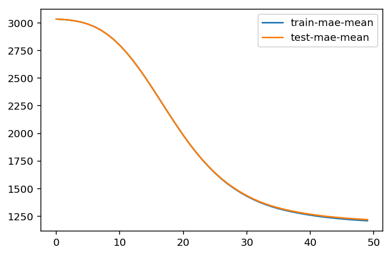
%%time

bst_cv1 = xgb.cv(xgb_params, dtrain, num_boost_round=50, nfold=3, seed=0, 
                feval=xg_eval_mae, maximize=False, early_stopping_rounds=10)

print ('CV score:', bst_cv1.iloc[-1,:]['test-mae-mean'])   #[-1,:] Take the last element

CV score: 1220.054769
CPU times: user 2min 24s, sys: 1.54 s, total: 2min 25s
Wall time: 2min 26s
We have the first baseline result: MAE=1218.9

plt.figure()
bst_cv1[['train-mae-mean', 'test-mae-mean']].plot()

2.3 First Base Model

In the tree model above:

Fitting did not occur
Only 50 tree models have been built

%%time
#Building 100 tree models
bst_cv2 = xgb.cv(xgb_params, dtrain, num_boost_round=100, 
                nfold=3, seed=0, feval=xg_eval_mae, maximize=False, 
                early_stopping_rounds=10)

print ('CV score:', bst_cv2.iloc[-1,:]['test-mae-mean'])

CV score: 1171.2875569999999
CPU times: user 4min 47s, sys: 2.05 s, total: 4min 49s
Wall time: 4min 51s

fig, (ax1, ax2) = plt.subplots(1,2)
fig.set_size_inches(16,4)
#100 trees
ax1.set_title('100 rounds of training')
ax1.set_xlabel('Rounds')
ax1.set_ylabel('Loss')
ax1.grid(True)
ax1.plot(bst_cv2[['train-mae-mean', 'test-mae-mean']])
ax1.legend(['Training Loss', 'Test Loss'])
#Last 60 Trees
ax2.set_title('60 last rounds of training')
ax2.set_xlabel('Rounds')
ax2.set_ylabel('Loss')
ax2.grid(True)
ax2.plot(bst_cv2.iloc[40:][['train-mae-mean', 'test-mae-mean']])
ax2.legend(['Training Loss', 'Test Loss'])

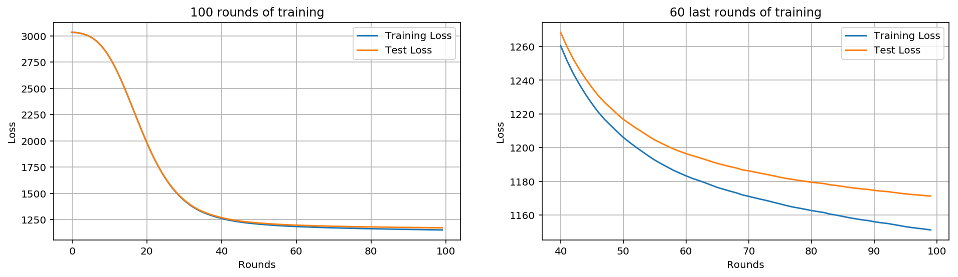
There's so little fitting going on, it's not that important yet

We've got a new record MAE = 1171.77 which is better than the first one (1218.9). Next we'll change the other parameters.

2.4 Xgboost Parameter Adjustment

Step 1: Select a set of initial parameters
Step 2: Change max_depth and min_child_weight.
Step 3: Adjusting gamma reduces the risk of model overfitting.
Step 4: Adjust subsample and colsample_bytree to change data sampling strategy.
Step 5: Adjust learning rate eta.

class XGBoostRegressor(object):
    def __init__(self, **kwargs):
        self.params = kwargs
        if 'num_boost_round' in self.params:
            self.num_boost_round = self.params['num_boost_round']
        self.params.update({'silent': 1, 'objective': 'reg:linear', 'seed': 0})
    #Training model    
    def fit(self, x_train, y_train):
        dtrain = xgb.DMatrix(x_train, y_train)
        self.bst = xgb.train(params=self.params, dtrain=dtrain, num_boost_round=self.num_boost_round,
                             feval=xg_eval_mae, maximize=False)
        
    def predict(self, x_pred):
        dpred = xgb.DMatrix(x_pred)
        return self.bst.predict(dpred)
    
    def kfold(self, x_train, y_train, nfold=5):
        dtrain = xgb.DMatrix(x_train, y_train)
        cv_rounds = xgb.cv(params=self.params, dtrain=dtrain, num_boost_round=self.num_boost_round,
                           nfold=nfold, feval=xg_eval_mae, maximize=False, early_stopping_rounds=10)
        return cv_rounds.iloc[-1,:]
    
    def plot_feature_importances(self):
        feat_imp = pd.Series(self.bst.get_fscore()).sort_values(ascending=False)
        feat_imp.plot(title='Feature Importances')
        plt.ylabel('Feature Importance Score')
        
    def get_params(self, deep=True):
        return self.params
 
    def set_params(self, **params):
        self.params.update(params)
        return self

#Evaluation Indicators
def mae_score(y_true, y_pred):
    return mean_absolute_error(np.exp(y_true), np.exp(y_pred))

mae_scorer = make_scorer(mae_score, greater_is_better=False)  #make_scorer

bst = XGBoostRegressor(eta=0.1, colsample_bytree=0.5, subsample=0.5, 
                       max_depth=5, min_child_weight=3, num_boost_round=50)

bst.kfold(train_x, train_y, nfold=5)

test-mae-mean 1218.528027
test-mae-std 10.423910
test-rmse-mean 0.562570
test-rmse-std 0.002914
train-mae-mean 1209.757422
train-mae-std 2.306814
train-rmse-mean 0.558842
train-rmse-std 0.000475
Name: 49, dtype: float64

Step 1: Learning Rate and Number of Trees

Step 2: Tree Depth and Node Weight
These parameters have the greatest impact on xgboost performance, so they should adjust first.We briefly outline them:

max_depth: The maximum depth of a tree.Increasing this value will make the model more complex and prone to fitting, and a depth of 3-10 is reasonable.
min_child_weight: Regularization parameter. Stops the tree building process if the instance weight in the tree partition is less than the defined sum.

xgb_param_grid = {'max_depth': list(range(4,9)), 'min_child_weight': list((1,3,6))}
xgb_param_grid['max_depth']

%%time
 
grid = GridSearchCV(XGBoostRegressor(eta=0.1, num_boost_round=50, colsample_bytree=0.5, subsample=0.5),
                param_grid=xgb_param_grid, cv=5, scoring=mae_scorer)

grid.fit(train_x, train_y.values)

grid.cv_results_, grid.best_params_, grid.best_score_

Best results from grid search:

{'max_depth': 8, 'min_child_weight': 6},
-1187.9597499123447)

Set to negative because you are looking for a large value

Step 3: Adjusting gamma to reduce the risk of over-fitting

%%time

xgb_param_grid = {'gamma':[ 0.1 * i for i in range(0,5)]}

grid = GridSearchCV(XGBoostRegressor(eta=0.1, num_boost_round=50, max_depth=8, min_child_weight=6,
                                        colsample_bytree=0.5, subsample=0.5),
                    param_grid=xgb_param_grid, cv=5, scoring=mae_scorer)

grid.fit(train_x, train_y.values)

grid.grid_scores_, grid.best_params_, grid.best_score_

([mean: -1187.95975, std: 6.71340, params: {'gamma': 0.0},
mean: -1187.67788, std: 6.44332, params: {'gamma': 0.1},
mean: -1187.66616, std: 6.75004, params: {'gamma': 0.2},
mean: -1187.21835, std: 7.06771, params: {'gamma': 0.30000000000000004},
mean: -1188.35004, std: 6.50057, params: {'gamma': 0.4}],
{'gamma': 0.30000000000000004},
-1187.2183540791846)

We chose to use a smaller gamma.

Step 4: Adjust sample sampling subsample and colsample_bytree

%%time

xgb_param_grid = {'subsample':[ 0.1 * i for i in range(6,9)],
                      'colsample_bytree':[ 0.1 * i for i in range(6,9)]}


grid = GridSearchCV(XGBoostRegressor(eta=0.1, gamma=0.2, num_boost_round=50, max_depth=8, min_child_weight=6),
                    param_grid=xgb_param_grid, cv=5, scoring=mae_scorer)
grid.fit(train_x, train_y.values)

grid.grid_scores_, grid.best_params_, grid.best_score_

([mean: -1185.67108, std: 5.40097, params: {'colsample_bytree': 0.6000000000000001, 'subsample': 0.6000000000000001},
mean: -1184.90641, std: 5.61239, params: {'colsample_bytree': 0.6000000000000001, 'subsample': 0.7000000000000001},
mean: -1183.73767, std: 6.15639, params: {'colsample_bytree': 0.6000000000000001, 'subsample': 0.8},
mean: -1185.09329, std: 7.04215, params: {'colsample_bytree': 0.7000000000000001, 'subsample': 0.6000000000000001},
mean: -1184.36149, std: 5.71298, params: {'colsample_bytree': 0.7000000000000001, 'subsample': 0.7000000000000001},
mean: -1183.83446, std: 6.24654, params: {'colsample_bytree': 0.7000000000000001, 'subsample': 0.8},
mean: -1184.43055, std: 6.68009, params: {'colsample_bytree': 0.8, 'subsample': 0.6000000000000001},
mean: -1183.33878, std: 5.74989, params: {'colsample_bytree': 0.8, 'subsample': 0.7000000000000001},
mean: -1182.93099, std: 5.75849, params: {'colsample_bytree': 0.8, 'subsample': 0.8}],
{'colsample_bytree': 0.8, 'subsample': 0.8},
-1182.9309918891634)

_, scores =  convert_grid_scores(grid.grid_scores_)
scores = scores.reshape(3,3)

plt.figure(figsize=(10,5))
cp = plt.contourf(xgb_param_grid['subsample'], xgb_param_grid['colsample_bytree'], scores, cmap='BrBG')
plt.colorbar(cp)
plt.title('Subsampling params tuning')
plt.annotate('Optimum', xy=(0.895, 0.6), xytext=(0.8, 0.695), arrowprops=dict(facecolor='black'))
plt.xlabel('subsample')
plt.ylabel('colsample_bytree')
plt.grid(True)
plt.show()

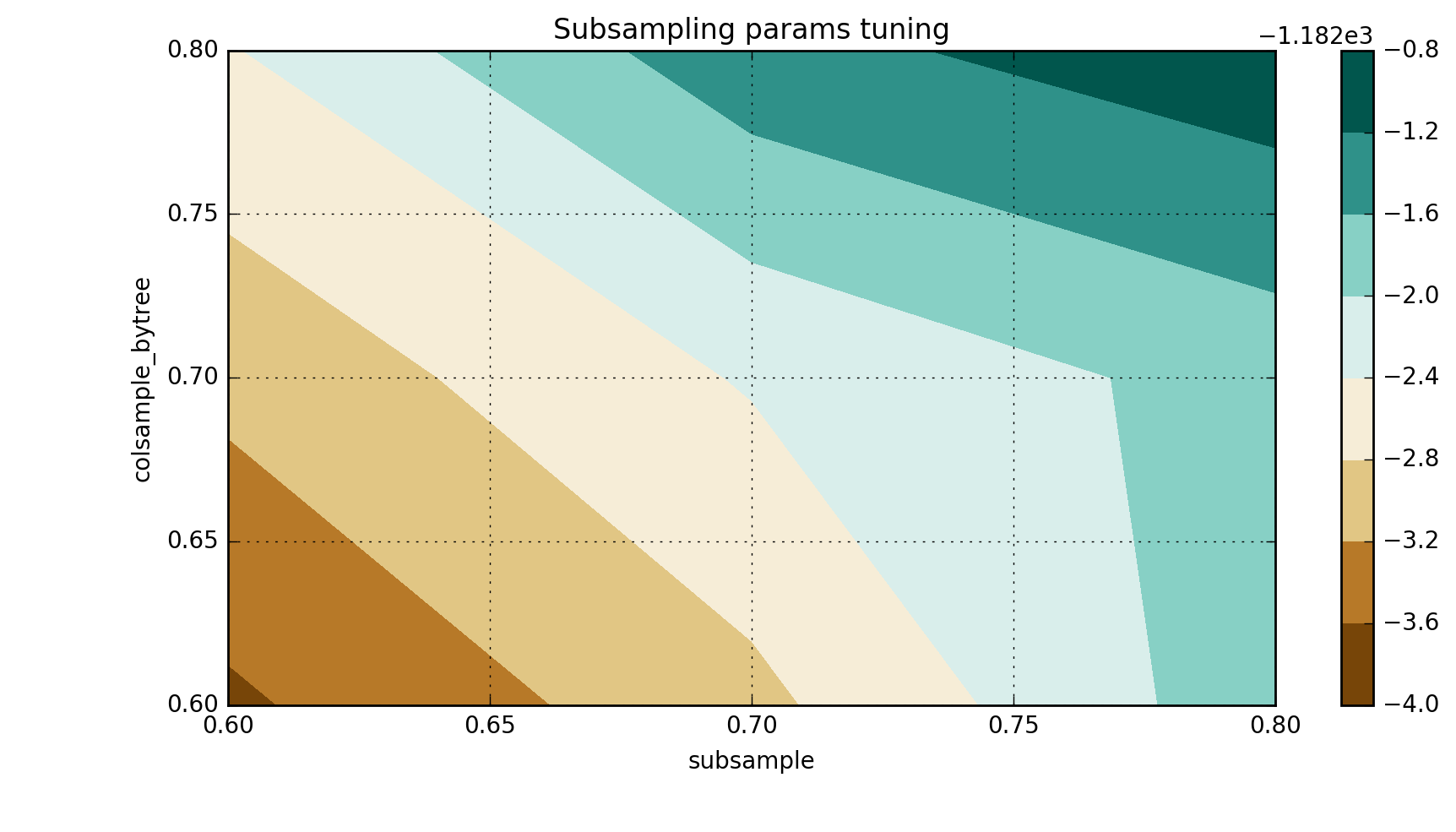
In the specific case of the current pre-training mode, I get the following results:

`{'colsample_bytree': 0.8, 'subsample': 0.8}, -1182.9309918891634)

Step 5: Reduce learning rate and increase number of trees

The final step in parameter optimization is to slow down learning while increasing more estimates.

1. First we iterate over 50 trees

%%time
    
xgb_param_grid = {'eta':[0.5,0.4,0.3,0.2,0.1,0.075,0.05,0.04,0.03]}
grid = GridSearchCV(XGBoostRegressor(num_boost_round=50, gamma=0.2, max_depth=8, min_child_weight=6,
                                        colsample_bytree=0.6, subsample=0.9),
                    param_grid=xgb_param_grid, cv=5, scoring=mae_scorer)

grid.fit(train_x, train_y.values)

grid.grid_scores_, grid.best_params_, grid.best_score_

([mean: -1205.85372, std: 3.46146, params: {'eta': 0.5},
mean: -1185.32847, std: 4.87321, params: {'eta': 0.4},
mean: -1170.00284, std: 4.76399, params: {'eta': 0.3},
mean: -1160.97363, std: 6.05830, params: {'eta': 0.2},
mean: -1183.66720, std: 6.69439, params: {'eta': 0.1},
mean: -1266.12628, std: 7.26130, params: {'eta': 0.075},
mean: -1709.15130, std: 8.19994, params: {'eta': 0.05},
mean: -2104.42708, std: 8.02827, params: {'eta': 0.04},
mean: -2545.97334, std: 7.76440, params: {'eta': 0.03}],
{'eta': 0.2},
-1160.9736284869114)

eta, y = convert_grid_scores(grid.grid_scores_)
plt.figure(figsize=(10,4))
plt.title('MAE and ETA, 50 trees')
plt.xlabel('eta')
plt.ylabel('score')
plt.plot(eta, -y)
plt.grid(True)
plt.show()

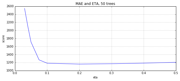
{'eta': 0.2}, -1160.9736284869114 is currently the best result

2. Now let's increase the tree to 100

xgb_param_grid = {'eta':[0.5,0.4,0.3,0.2,0.1,0.075,0.05,0.04,0.03]}
grid = GridSearchCV(XGBoostRegressor(num_boost_round=100, gamma=0.2, max_depth=8, min_child_weight=6,
                                        colsample_bytree=0.6, subsample=0.9),
                    param_grid=xgb_param_grid, cv=5, scoring=mae_scorer)

grid.fit(train_x, train_y.values)

grid.grid_scores_, grid.best_params_, grid.best_score_

([mean: -1231.04517, std: 5.41136, params: {'eta': 0.5},
mean: -1201.31398, std: 4.75456, params: {'eta': 0.4},
mean: -1177.86344, std: 3.67324, params: {'eta': 0.3},
mean: -1160.48853, std: 5.65336, params: {'eta': 0.2},
mean: -1152.24715, std: 5.85286, params: {'eta': 0.1},
mean: -1156.75829, std: 5.30250, params: {'eta': 0.075},
mean: -1184.88913, std: 6.08852, params: {'eta': 0.05},
mean: -1243.60808, std: 7.40326, params: {'eta': 0.04},
mean: -1467.04736, std: 8.70704, params: {'eta': 0.03}],
{'eta': 0.1},
-1152.2471498726127)

eta, y = convert_grid_scores(grid.grid_scores_)
plt.figure(figsize=(10,4))
plt.title('MAE and ETA, 100 trees')
plt.xlabel('eta')
plt.ylabel('score')
plt.plot(eta, -y)
plt.grid(True)
plt.show()

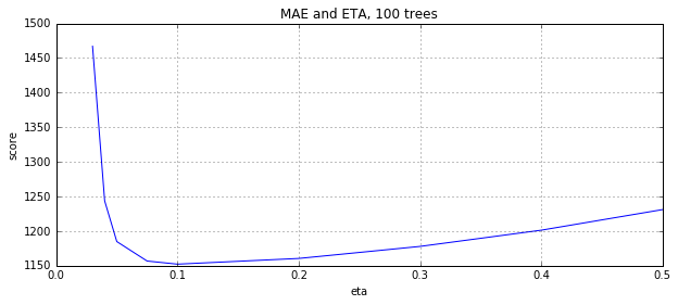
A lower learning rate has better results

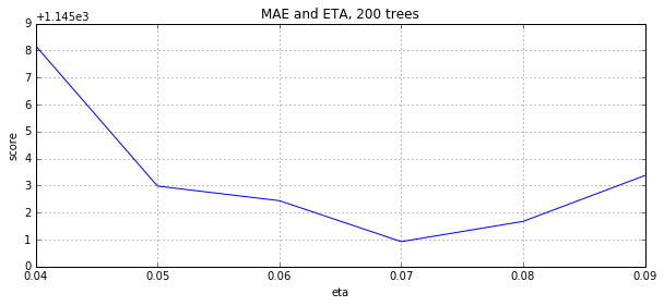
3. Continue to increase the number of trees to 200

%%time

xgb_param_grid = {'eta':[0.09,0.08,0.07,0.06,0.05,0.04]}
grid = GridSearchCV(XGBoostRegressor(num_boost_round=200, gamma=0.2, max_depth=8, min_child_weight=6,
                                        colsample_bytree=0.6, subsample=0.9),
                    param_grid=xgb_param_grid, cv=5, scoring=mae_scorer)

grid.fit(train_x, train_y.values)

grid.grid_scores_, grid.best_params_, grid.best_score_

([mean: -1148.37246, std: 6.51203, params: {'eta': 0.09},
mean: -1146.67343, std: 6.13261, params: {'eta': 0.08},
mean: -1145.92359, std: 5.68531, params: {'eta': 0.07},
mean: -1147.44050, std: 6.33336, params: {'eta': 0.06},
mean: -1147.98062, std: 6.39481, params: {'eta': 0.05},
mean: -1153.17886, std: 5.74059, params: {'eta': 0.04}],
{'eta': 0.07},
-1145.9235944370419)

eta, y = convert_grid_scores(grid.grid_scores_)
plt.figure(figsize=(10,4))
plt.title('MAE and ETA, 200 trees')
plt.xlabel('eta')
plt.ylabel('score')
plt.plot(eta, -y)
plt.grid(True)
plt.show()

3 Summary

%%time

# Final XGBoost model


bst = XGBoostRegressor(num_boost_round=200, eta=0.07, gamma=0.2, max_depth=8, min_child_weight=6,
                                        colsample_bytree=0.6, subsample=0.9)
cv = bst.kfold(train_x, train_y, nfold=5)

cv

test-mae-mean 1146.997852
test-mae-std 9.541592
train-mae-mean 1036.557251
train-mae-std 0.974437
Name: 199, dtype: float64

We see that the best ETA for 200 trees is 0.07.As we expected, the ETA and num_boost_round dependencies are not linear, but there are some associations.

They spent a considerable amount of time optimizing xgboost. From the initial value: 1219.57. After tuning, they reached MAE=1171.77.

We also found a relationship between ETA and num_boost_round:

100 trees, eta=0.1: MAE=1152.247
200 trees, eta=0.07: MAE=1145.92

`XGBoostRegressor(num_boost_round=200, gamma=0.2, max_depth=8, min_child_weight=6, colsample_bytree=0.6, subsample=0.9, eta=0.07).

one named slash

90 original articles published. 60% praised. 90,000 visits+

Private letter follow

Posted by rimelta on Wed, 11 Mar 2020 21:00:47 -0700

Programmer Group