1. Emotional Analysis of Chinese Comments (keras+rnn)

1.1 Required Libraries

# First load the required libraries, jieba and gensim are in Chinese only 
# The%matplotlib inline function allows inline drawing and omits the plt.show() step
%matplotlib inline 
import numpy as np
import matplotlib.pyplot as plt
import re #Regularization
import jieba # Chinese must be used as computer does not break sentences
# gensim is used to load pre-training word vector
from gensim.models import KeyedVectors
#KeyedVectors map entities (words, documents, pictures can all) to vectors, all represented by string IDS
#Sometimes there are many warning outputs when running code, such as reminding a new version, if you don't want to mess up the output
import warnings
warnings.filterwarnings("ignore")

1.2 Pre-training Word Vector

Word bag cn_model: The open source link of "chinese-word-vectors" github by Institute of Chinese Information Processing of Beijing Normal University and researcher of DBIIR Laboratory of People's University of China is https://github.com/Embedding/Chinese-Word-Vectors.Here we use the word vector of "chinese-word-vectors" known as Word + Ngram, which can be downloaded from the GitHub link above. The author himself downloads it to the networking disk and other corpus and needs to establish his own reading path. Link: https://pan.baidu.com/s/1RCrNNAagOjLq0BP8cA9EQ Extraction Code: fgux

# Loading pre-training Chinese participle embedding using gensim
cn_model = KeyedVectors.load_word2vec_format('chinese_word_vectors/sgns.zhihu.bigram', 
                                          binary=False)

1.3 Word Vector Model

In this word vector model, each word is an index, corresponding to a vector with a length of 300. The LSTM neural network model that we need to build today does not directly process the Chinese character text. It needs to be graded and converted into word vector first. Steps refer to: 0. Original text: I like literature 1. Word breaking: I, like, literature2.Tokenize (indexed): [2,345,4564] 3.Embedding (word vectorization): with a 300-dimensional word vector, the above tokens become a [3,300] matrix 4.RNN:1 DCONV, GRU, LSTM, etc. 5.Classified by activation function output: e.g., sigmoid output between 0 and 1

# So each word corresponds to a vector of 300 lengths
embedding_dim = cn_model['Shandong University'].shape[0]  #shape[0] returns rows
print('The length of the word vector is{}'.format(embedding_dim))
cn_model['Shandong University']

The output is as follows

The length of the word vector is 300
Out[3]:
array([-2.603470e-01, 3.677500e-01, -2.379650e-01, 5.301700e-02,
-3.628220e-01, -3.212010e-01, -1.903330e-01, 1.587220e-01,
.
dtype=float32)

# Compute Similarity
cn_model.similarity('A mandarin orange', 'orange')

output

# dot ('orange'/|'orange'|,'orange'/|'orange'|), cosine similarity
np.dot(cn_model['A mandarin orange']/np.linalg.norm(cn_model['A mandarin orange']), 
cn_model['orange']/np.linalg.norm(cn_model['orange']))

output

# Find the closest word, cosine similarity
cn_model.most_similar(positive=['University?'], topn=10)

output

# Find out different words
test_words = 'Teacher Accountant Programmer Lawyer Doctor Elderly'
test_words_result = cn_model.doesnt_match(test_words.split())
print('stay '+test_words+' in:\n Words that are not of the same category are: %s' %test_words_result)

output

cn_model.most_similar(positive=['woman','Derail'], negative=['Man'], topn=1)

output

1.4 Training corpus (dataset)

This tutorial uses Hotel reviews, where training samples are placed in two folders: pos and neg, with 2000 txt files in each folder, a comment in each file, and 4000 training samples. Sample data of this size is very minimal in the NLP

# Get an index of the samples, which are stored in two folders.
# Positive evaluation'pos'folder and negative evaluation'neg' folder, respectively
# There are 2,000 txt files in each folder, one for each evaluation
import os #Read-in Read-out Channel
pos_txts = os.listdir('pos')
neg_txts = os.listdir('neg')

print( 'Total Samples: '+ str(len(pos_txts) + len(neg_txts)) )

# Now let's put all the reviews in a list
train_texts_orig = [] # Store all reviews, one string per case, original review
# After adding all the samples, train_texts_orig is a list of 4000 texts
# Among them, the first 2000 texts are positive and the last 2000 are negative.
#Following is the process of reading in the.txt file
for i in range(len(pos_txts)):
    with open('pos/'+pos_txts[i], 'r', errors='ignore') as f:
        text = f.read().strip()
        train_texts_orig.append(text)
        f.close()
for i in range(len(neg_txts)):
    with open('neg/'+neg_txts[i], 'r', errors='ignore') as f:
        text = f.read().strip()
        train_texts_orig.append(text)
        f.close()

len(train_texts_orig)

# We use tensorflow's keras interface to model
from keras.models import Sequential
from keras.layers import Dense, GRU, Embedding, LSTM, Bidirectional#Dense Full Connection
#Bidirectional bidirectional LSTM callbacks are used to tune parameters
from keras.preprocessing.text import Tokenizer
from keras.preprocessing.sequence import pad_sequences
from keras.optimizers import RMSprop
from keras.optimizers import Adam
from keras.callbacks import EarlyStopping, ModelCheckpoint, TensorBoard, ReduceLROnPlateau

1.5 participle and tokenize

First we remove the punctuation from each sample, and then we use the jieba participle, which returns a generator. It is not possible to directly tokenize the result, so we convert the participle result into a list and index it so that each evaluated text becomes an index number corresponding to the words in the pre-training words Vector model.

# Perform word segmentation and tokenize
# train_tokens is a long list with 4,000 small lists for each evaluation
train_tokens = []
for text in train_texts_orig:
    # Remove punctuation
    text = re.sub("[\s+\.\!\/_,$%^*(+\"\']+|[+-!，. ？,~@#￥%......&*()]+", "",text)
    # Stubborn participle
    cut = jieba.cut(text)
    # The output of a stuttering participle is a generator
    # Convert generator to list
    cut_list = [ i for i in cut ]
    for i, word in enumerate(cut_list):
        try:
            # Convert words to index
            cut_list[i] = cn_model.vocab[word].index
        except KeyError:
            # If the word is not in the dictionary, output 0
            cut_list[i] = 0
    train_tokens.append(cut_list)

1.6 Index Length Standardization

Because the length of each comment is not the same, if we simply take the longest comment and fill the other with the same length, it would be a waste of computing resources, so we take a compromise length.

# Get the length of all tokens
num_tokens = [ len(tokens) for tokens in train_tokens ]
num_tokens = np.array(num_tokens)

# Average tokens length
np.mean(num_tokens)

# Length of longest evaluation tokens
np.max(num_tokens)

plt.hist(np.log(num_tokens), bins = 100)#Has logarithm of size
plt.xlim((0,20))
plt.ylabel('number of tokens')
plt.xlabel('length of tokens')
plt.title('Distribution of tokens length')
plt.show()

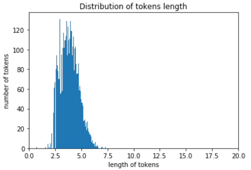
# Take the average tokens and add the standard deviation of two tokens.
# Assuming that the distribution of tokens length is normal, the value max_tokens can cover about 95% of the samples
max_tokens = np.mean(num_tokens) + 2 * np.std(num_tokens)
max_tokens = int(max_tokens)
max_tokens

# When the length of tokens is 236, about 95% of the samples are covered
# We padding the lengths that are insufficient and trimming the lengths that are too long
np.sum( num_tokens < max_tokens ) / len(num_tokens)

1.7 Reverse tokenize

To verify later, we define a function to convert the index into readable text, which is important for debug.

# Used to convert tokens to text
def reverse_tokens(tokens):
    text = ''
    for i in tokens:
        if i != 0:
            text = text + cn_model.index2word[i]
        else:
            text = text + ' '
    return text

reverse = reverse_tokens(train_tokens[0])

# Restore to text after tokenize
# No more punctuation visible
reverse

# Original Text
train_texts_orig[0]

1.8 Building an embedding matrix

Now let's prepare the embedding matrix for the model. According to keras, we need to prepare a dimension of (numwords,Matrix of embeddingdim [num words stands for the number of words we use, EmdeddingDimension is 300 in the pre-training word vector model we are using now, and each word is represented by a vector with a length of 300.) Note that we only select the first 50 K most frequently used words. In this pre-training word vector model, there are 2.6 million vocabularies, which would be a waste of computational resources if used entirely on classification issues, because our training samples are very smallSmall, there is only 4k in total. If we have 100k, 200k or more training samples, we can consider reducing the vocabulary used in classification.

embedding_dim

# Use only the first 50,000 words in the library
num_words = 50000
# Initialize embedding_matrix and apply on keras
embedding_matrix = np.zeros((num_words, embedding_dim))
# embedding_matrix is a [num_words, embedding_dim] matrix
# Dimension 50000 * 300
for i in range(num_words):
    embedding_matrix[i,:] = cn_model[cn_model.index2word[i]]
embedding_matrix = embedding_matrix.astype('float32')

# Check if the index corresponds,
# Output 300 means that embedding vectors of length 300 correspond one-to-one
np.sum( cn_model[cn_model.index2word[333]] == embedding_matrix[333] )

# The dimension of embedding_matrix,
# This dimension is required by keras and will be used later in the model
embedding_matrix.shape

1.9 padding and truncating

After converting the text to tokens, the length of each index string is not equal, so we need to standardize the length of the index to facilitate the training of the model. We chose 236 above, which can cover 95% of the training samples. Next we padding and truncating. We usually use the'pre'method, which is in front of the text index.Fill in 0 because, according to some research practice, filling in 0 after the text index can have some adverse effects on the model.

# For padding and truncating, the input train_tokens is a list
# The returned train_pad is a numpy array
train_pad = pad_sequences(train_tokens, maxlen=max_tokens,
                            padding='pre', truncating='pre')

# Replace words exceeding 50,000 word vectors with 0
train_pad[ train_pad>=num_words ] = 0

# You can see that after padding the tokens before become all 0, and the text is at the end
train_pad[33]

array([ 0, 0, 0, 0, 0, 0, 0, 0, 0,
0, 0, 0, 0, 0, 0, 0, 0, 0,
0, 0, 0, 0, 0, 0, 0, 0, 0,
0, 0, 0, 0, 0, 0, 0, 0, 0,
0, 0, 0, 0, 0, 0, 0, 0, 0,
0, 0, 0, 0, 0, 0, 0, 0, 0,
0, 0, 0, 0, 0, 0, 0, 0, 0,
0, 0, 0, 0, 0, 0, 0, 0, 0,
0, 0, 0, 0, 0, 0, 0, 0, 0,
0, 0, 0, 0, 0, 0, 0, 0, 0,
0, 0, 0, 0, 0, 0, 0, 0, 0,
0, 0, 0, 0, 0, 0, 0, 0, 0,
0, 0, 0, 0, 0, 0, 0, 0, 0,
0, 0, 0, 0, 0, 0, 0, 0, 0,
0, 0, 0, 0, 0, 0, 0, 0, 0,
0, 0, 0, 0, 0, 0, 0, 0, 0,
0, 0, 0, 0, 0, 0, 0, 0, 0,
290, 3053, 57, 169, 73, 1, 25, 11216, 49,
163, 15985, 0, 0, 30, 8, 0, 1, 228,
223, 40, 35, 653, 0, 5, 1642, 29, 11216,
2751, 500, 98, 30, 3159, 2225, 2146, 371, 6285,
169, 27396, 1, 1191, 5432, 1080, 20055, 57, 562,
1, 22671, 40, 35, 169, 2567, 0, 42665, 7761,
110, 0, 0, 41281, 0, 110, 0, 35891, 110,
0, 28781, 57, 169, 1419, 1, 11670, 0, 19470,
1, 0, 0, 169, 35071, 40, 562, 35, 12398,
657, 4857])

# Prepare the target vector, the first 2000 samples are 1, and the last 2000 are 0
train_target = np.concatenate( (np.ones(2000),np.zeros(2000)) )

# Segmentation of training and test samples
from sklearn.model_selection import train_test_split

train_target.shape
train_pad.shape

# 90% of the samples were used for training and the remaining 10% for testing
#Since the first 2,000 folders are in the neg category, scramble the order to train random_state
X_train, X_test, y_train, y_test = train_test_split(train_pad,
                                                    train_target,
                                                    test_size=0.1,
                                                    random_state=12
                                                    )

# Check training samples to make sure they are correct
print(reverse_tokens(X_train[35]))
print('class: ',y_train[35])

1.10 Building LSTM Model with Keas

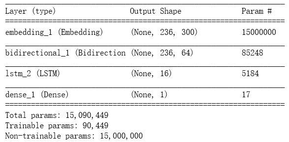
The first layer of the model is the Embedding layer. Text can only be processed with a neural network when we convert the tokens index to a word vector matrix.Keas provides an Embedding interface to avoid tedious sparse matrix operations.At the Embedding layer we enter the following matrix: (batchsize, maxtokens) and the output matrix is: (batchsize, maxtokens, embeddingdim)

# Classifying samples using LSTM
model = Sequential()

# The first layer of the model is embedding, trainable=False because embedding_matrix has been trained since it was downloaded
model.add(Embedding(num_words,
                    embedding_dim,
                    weights=[embedding_matrix],
                    input_length=max_tokens,
                    trainable=False))

model.add(Bidirectional(LSTM(units=32, return_sequences=True)))#Bidirectional LSTM considers both before and after words
model.add(LSTM(units=16, return_sequences=False))#units=16 neurons

GRU: If you use GRU, the test sample can achieve 87% accuracy, but when I test my own text content, I find that the output of the last activation function of GRU is around 0.5, which indicates that the judgment of the model is not clear, confidence is low, and it is found that the judgment of the model on negative sentences can sometimes be wrong after testing. We expect the output of negative samples to be close to 0, positive sampleBen is close to 1 instead of hovering between 0.5.
BILSTM: Tested LSTM and BiLSTM, found that BiLSTM performed best and LSTM performed slightly better than GRU because BiLSTM has better memory for longer sentence structures.After Embedding, the first layer uses BiLSTM to return sequences, then the second layer and the 16-unit LSTM do not return sequences, only the final result, and finally a full-link layer that uses the sigmoid activation function to output the results

# GRU Code
# model.add(GRU(units=32, return_sequences=True))
# model.add(GRU(units=16, return_sequences=True))
# model.add(GRU(units=4, return_sequences=False))

#Add Full Connection Layer
model.add(Dense(1, activation='sigmoid'))
# We used adam to optimize with 0.001 learning rate
optimizer = Adam(lr=1e-3)

model.compile(loss='binary_crossentropy',
              optimizer=optimizer,  
              metrics=['accuracy'])

# Let's look at the structure of the model. There are about 90k trainable variables. None means batchsize. A batch has 236 words in it
#15000000 is 50000*300, because train=false, these parameters are not trained
#17=16*1+1(bias is a parameter)
model.summary()

# Create a storage point for weights, verbose=1 can print more detailed information, look for problems
path_checkpoint = 'sentiment_checkpoint.keras'
checkpoint = ModelCheckpoint(filepath=path_checkpoint, monitor='val_loss',
                                      verbose=1, save_weights_only=True,
                                      save_best_only=True)

# Attempting to load a trained model
try:
    model.load_weights(path_checkpoint)
except Exception as e:
    print(e)

# Define early stoping to stop training if validation loss does not improve within 3 epoch s
earlystopping = EarlyStopping(monitor='val_loss', patience=3, verbose=1)

# Automatically reduce learning rate
lr_reduction = ReduceLROnPlateau(monitor='val_loss',
                                       factor=0.1, min_lr=1e-5, patience=0,
                                       verbose=1)

# Define callback function
callbacks = [
    earlystopping, 
    checkpoint,
    lr_reduction
]

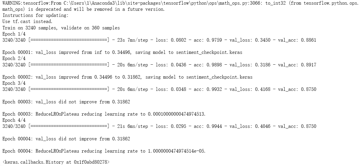
# Start training, 4000*0.1=400 as test, validation_split=0.1 as 3600*0.1
model.fit(X_train, y_train,
          validation_split=0.1, 
          epochs=4,
          batch_size=128,
          callbacks=callbacks)

1.11 Conclusion

We define a prediction function (processing and re-entering the input text as required by the model) to predict the polarity of the input text, so that the model can accurately judge negative sentences and some simple logical structures.

result = model.evaluate(X_test, y_test)
print('Accuracy:{0:.2%}'.format(result[1]))

def predict_sentiment(text):
    print(text)
    # Depunctuation
    text = re.sub("[\s+\.\!\/_,$%^*(+\"\']+|[+-!，. ？,~@#￥%......&*()]+", "",text)
    # participle
    cut = jieba.cut(text)
    cut_list = [ i for i in cut ]
    # tokenize
    for i, word in enumerate(cut_list):
        try:
            cut_list[i] = cn_model.vocab[word].index
        except KeyError:
            cut_list[i] = 0
    # padding
    tokens_pad = pad_sequences([cut_list], maxlen=max_tokens,
                           padding='pre', truncating='pre')
    # Forecast
    result = model.predict(x=tokens_pad)
    coef = result[0][0]
    if coef >= 0.5:
        print('Is a positive evaluation','output=%.2f'%coef)
    else:
        print('Is a negative evaluation','output=%.2f'%coef)

test_list = [
    'Hotel facilities are not new and service attitudes are poor',
    'The room is cool with plenty of air conditioning',
    'The hotel environment is not good and the accommodation experience is not good',
    'Insufficient room insulation' ,
    'Come back in the evening and find no cleaning'   
]
for text in test_list:
    predict_sentiment(text)

1.12 Misclassification

y_pred = model.predict(X_test)
y_pred = y_pred.T[0]
y_pred = [1 if p>= 0.5 else 0 for p in y_pred]
y_pred = np.array(y_pred)

y_actual = np.array(y_test)

# Find index for misclassification
misclassified = np.where( y_pred != y_actual )[0]

# Output all misclassified indexes, 48 out of 400 tests
len(misclassified)
print(len(misclassified))

# Let's find a sample of misclassified errors. misclassified[1] made the second mistake.
idx=misclassified[1]
print(reverse_tokens(X_test[idx]))
print('Classification of predictions', y_pred[idx])
print('Actual Classification', y_actual[idx])

2. Sina News Category (tensorflow+cnn)

The dataset uses the author of the Tsinghua dataset to intercept part of the dataset, Baidu cloud download link:
Link: https://pan.baidu.com/s/1-Rm9PU7ekU3zx_7gTB9ibw Extraction Code: 3d3o

#Here's how to get the file
import os
def getFilePathList(rootDir):
    filePath_list = []
    for walk in os.walk(rootDir):
        part_filePath_list = [os.path.join(walk[0], file) for file in walk[2]]
        filePath_list.extend(part_filePath_list)
    return filePath_list
filePath_list = getFilePathList('part_cnews')
len(filePath_list)#A total of 1400.txt files make up a list

Run result:

filePath_list[5]

Run result: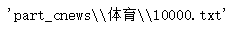

#All sample label values are summarized into a list and assigned to label_list
#windows differs from Linux system path strings by the interval character
label_list = []
for filePath in filePath_list:
    label = filePath.split('\\')[1]
    label_list.append(label)
len(label_list)

Run result:

#Label Statistics Count
import pandas as pd 
pd.value_counts(label_list)

Run result: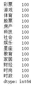

#Save label_list with the pickle Library
import pickle
with open('label_list.pickle','wb') as file:
    pickle.dump(label_list,file)

#Get all sample content, save content_list
#Pile.dump persists objects in python to binary files, which load very quickly.Avoid memory overflow by using the dump method of the pickle library to save every number of files read
import time
import pickle
import re

def getFile(filePath):
   with open(filePath, encoding='utf8') as file:
       fileStr = ''.join(file.readlines(1000))
   return fileStr

interval = 100
n_samples = len(label_list)
startTime = time.time()
directory_name = 'content_list'
if not os.path.isdir(directory_name):
   os.mkdir(directory_name)
for i in range(0, n_samples, interval):
   startIndex = i
   endIndex = i + interval
   content_list = []
   print('%06d-%06d start' %(startIndex, endIndex))
   for filePath in filePath_list[startIndex:endIndex]:
       fileStr = getFile(filePath)
       content = re.sub('\s+', ' ', fileStr)
       content_list.append(content)
   save_fileName = directory_name + '/%06d-%06d.pickle' %(startIndex, endIndex)
   with open(save_fileName, 'wb') as file:
       pickle.dump(content_list, file)
   used_time = time.time() - startTime
   print('%06d-%06d used time: %.2f seconds' %(startIndex, endIndex, used_time))

Run result: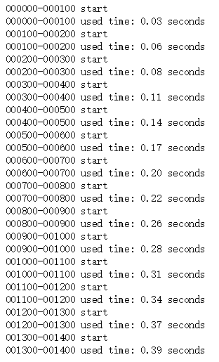

#Previously, in order to get the data and get the original data for processing, [content_list folder, label_list file, code file] are all in the same path
#Loading data
import time
import pickle
import os

def getFilePathList(rootDir):
    filePath_list = []
    for walk in os.walk(rootDir):
        part_filePath_list = [os.path.join(walk[0], file) for file in walk[2]]
        filePath_list.extend(part_filePath_list)
    return filePath_list

startTime = time.time()
contentListPath_list = getFilePathList('content_list')
content_list = []
for filePath in contentListPath_list:
    with open(filePath, 'rb') as file:
        part_content_list = pickle.load(file)
    content_list.extend(part_content_list)
with open('label_list.pickle', 'rb') as file:
    label_list = pickle.load(file)
used_time = time.time() - startTime
print('used time: %.2f seconds' %used_time)
sample_size = len(content_list)
print('length of content_list，mean sample size: %d' %sample_size)

Run result: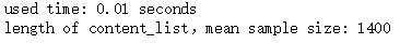

len(content_list)

Run result:

#Make a vocabulary: The elements in the content_list of the content list are the content of each article, and the data type is a string.
#Words in all articles are counted and the top 5000 occurrences are assigned to the variable vocabulary_list.
from collections import Counter 
def getVocabularyList(content_list, vocabulary_size):
    allContent_str = ''.join(content_list)
    counter = Counter(allContent_str)
    vocabulary_list = [k[0] for k in counter.most_common(vocabulary_size)]
    return ['PAD'] + vocabulary_list
startTime = time.time()
vocabulary_list = getVocabularyList(content_list, 5000)
used_time = time.time() - startTime
print('used time: %.2f seconds' %used_time)

Run result:

#Save vocabulary
import pickle 

with open('vocabulary_list.pickle', 'wb') as file:
    pickle.dump(vocabulary_list, file)

#Loading vocabularies: When you have finished making vocabularies, save them.Running the code afterwards directly loads the saved vocabulary, saving you time copying it as a vocabulary.
import pickle

with open('vocabulary_list.pickle', 'rb') as file:
    vocabulary_list = pickle.load(file)

#Data preparation
#Press Esc in the code block to enter command mode, and the vertical line to the left of the code block appears blue.In command mode, clicking the L key displays the number of lines of code
import time
startTime = time.time()#Record the start time of this code run and assign it to the variable startTime
from sklearn.model_selection import train_test_split
train_X, test_X, train_y, test_y = train_test_split(content_list, label_list)
train_content_list = train_X
train_label_list = train_y
test_content_list = test_X
test_label_list = test_y
used_time = time.time() - startTime #Print a prompt indicating how long it takes the program to run to this point
print('train_test_split used time : %.2f seconds' %used_time)

vocabulary_size = 10000  # Vocabulary expression is small
sequence_length = 600  # Sequence Length
embedding_size = 64  # Word vector dimension
num_filters = 256  # Number of convolution cores
filter_size = 5  # Convolution Kernel Size
num_fc_units = 128  # Full Junction Layer Neurons
dropout_keep_probability = 0.5  # dropout retention ratio
learning_rate = 1e-3  # learning rate
batch_size = 64  # Training size per batch

word2id_dict = dict([(b, a) for a, b in enumerate(vocabulary_list)])#Use list derivation to get a list of words and their id s, and call dict to cast the list into a dictionary
content2idList = lambda content : [word2id_dict[word] for word in content if word in word2id_dict]#Use list derivation and anonymous functions to define the function content2idlist, which converts every word in the article to an id
train_idlist_list = [content2idList(content) for content in train_content_list]#The result of the list derivation is a list of lists, with the elements in the total list train_id list_list being a list of IDS corresponding to the words in each article
used_time = time.time() - startTime#Code print prompt indicating how long it takes the program to run to this point
print('content2idList used time : %.2f seconds' %used_time)

import numpy as np
num_classes = np.unique(label_list).shape[0]#Gets the number of categories for a label, such as 14 for this article, where the value of the variable num_classes is 14
#The following six behaviors obtain a feature matrix and predictive target values that can be used for model training
import tensorflow.contrib.keras as kr
train_X = kr.preprocessing.sequence.pad_sequences(train_idlist_list, sequence_length)#The uniform length of each sample is seq_length, i.e. the superparameter above 600 has been set to 600
from sklearn.preprocessing import LabelEncoder#LaelEncoder method for importing sklearn.preprocessing Library
labelEncoder = LabelEncoder()#Instantiate LabelEncoder object
train_y = labelEncoder.fit_transform(train_label_list)#Call fit_transform method of LabelEncoder object for label encoding
train_Y = kr.utils.to_categorical(train_y, num_classes)#Call the to_categorical method of the keras.untils library to encode the result of label encoding before Ont-Hot encoding

import tensorflow as tf
tf.reset_default_graph()#Reset tensorflow diagram to enhance code robustness
X_holder = tf.placeholder(tf.int32, [None, sequence_length])
Y_holder = tf.placeholder(tf.float32, [None, num_classes])
used_time = time.time() - startTime
print('data preparation used time : %.2f seconds' %used_time)

Run result:

list(word2id_dict.items())[:20]

Run result: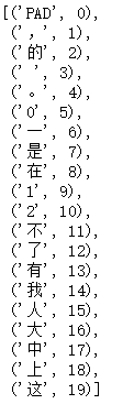

#Build Neural Network
embedding = tf.get_variable('embedding', 
                            [vocabulary_size, embedding_size])#Calling the get_variable method of the tf library to instantiate the updatable model parameter embedding, the matrix shape is vocabulary_size*embedding_size, or 10000*64
embedding_inputs = tf.nn.embedding_lookup(embedding,#By embedding the input data into words, the new variable embedding_inputs has the shape batch_size*sequence_length*embedding_size, or 64*600*64
                                          X_holder)
conv = tf.layers.conv1d(embedding_inputs,  #Calling the tf.layers.conv1d method requires three parameters, the first is the input data, the second is the number of convolution cores num_filters, and the third is the convolution core size filter_size
                        num_filters,       #The result of the method is assigned to the variable conv in the shape of batch_size*596*num_filters, 596 being the result of 600-5+1
                        filter_size)
max_pooling = tf.reduce_max(conv,  #Do a maximum operation on the first dimension of the variable conv.The result of the method is assigned to the variable max_pooling in the shape of batch_size*num_filters, or 64*256
                            [1])
full_connect = tf.layers.dense(max_pooling, #Add a full connection layer, and the result of the tf.layers.dense method is assigned to the variable full_connect in the shape of batch_size*num_fc_units, or 64*128
                               num_fc_units)
full_connect_dropout = tf.contrib.layers.dropout(full_connect, #The code calls the tf.contrib.layers.dropout method, which requires two parameters, the first is the input data and the second is the preservation ratio
                                                 keep_prob=dropout_keep_probability)
full_connect_activate = tf.nn.relu(full_connect_dropout) #Activation function
softmax_before = tf.layers.dense(full_connect_activate, #Add a full connection layer, and the result of the tf.layers.dense method is assigned to the variable softmax_before in the shape of batch_size*num_classes, or 64*14
                                 num_classes)
predict_Y = tf.nn.softmax(softmax_before)  #tf.nn.softmax method, the result of which is the prediction probability value
cross_entropy = tf.nn.softmax_cross_entropy_with_logits_v2(labels=Y_holder,
                                                           logits=softmax_before)
loss = tf.reduce_mean(cross_entropy)
optimizer = tf.train.AdamOptimizer(learning_rate)
train = optimizer.minimize(loss)
isCorrect = tf.equal(tf.argmax(Y_holder, 1), tf.argmax(predict_Y, 1))
accuracy = tf.reduce_mean(tf.cast(isCorrect, tf.float32))

#Parameter initialization is one of the most important parameters for neural network models.Initialization of parameters is required before training the neural network model
init = tf.global_variables_initializer()
session = tf.Session()
session.run(init)

#model training
test_idlist_list = [content2idList(content) for content in test_content_list] #Get data from test set
test_X = kr.preprocessing.sequence.pad_sequences(test_idlist_list, sequence_length)
test_y = labelEncoder.transform(test_label_list)
test_Y = kr.utils.to_categorical(test_y, num_classes)
import random
for i in range(100): #Model iteration training 100 times
    selected_index = random.sample(list(range(len(train_y))), k=batch_size)#Select batch_size from training set, that is, 64 samples for batch gradient reduction
    batch_X = train_X[selected_index]
    batch_Y = train_Y[selected_index]
    session.run(train, {X_holder:batch_X, Y_holder:batch_Y}) #Each run represents a model training session
    step = i + 1 
    if step % 10 == 0:#Print every 10 steps
        selected_index = random.sample(list(range(len(test_y))), k=100)#Randomly select 100 samples from a test set
        batch_X = test_X[selected_index]
        batch_Y = test_Y[selected_index]
        loss_value, accuracy_value = session.run([loss, accuracy], {X_holder:batch_X, Y_holder:batch_Y})
        print('step:%d loss:%.4f accuracy:%.4f' %(step, loss_value, accuracy_value))

Run result: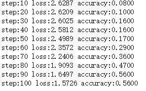

import warnings
warnings.filterwarnings("ignore")
def predict(input_content):
   #The data type of the idList must be a list list.
   #Otherwise, calling the kr.preprocessing.sequence.pad_sequences method will cause an error
   idList = [content2idList(input_content)]
   X = kr.preprocessing.sequence.pad_sequences(idList, sequence_length)
   Y = session.run(predict_Y, {X_holder:X})
   y = np.argmax(Y, axis=1)
   label = labelEncoder.inverse_transform(y)[0]
   return label

selected_index = random.sample(range(len(test_content_list)), k=1)[0]
selected_sample = test_content_list[selected_index]
true_label = test_label_list[selected_index]
predict_label = predict(selected_sample)

print('selected_sample :', selected_sample)
print('true_label :', true_label)
print('predict_label :', predict_label, '\n')
print('predict whatever you want, for example:')
input_content = "Football referee hits"
print('predict("%s") :' %input_content, predict(input_content))

Run result: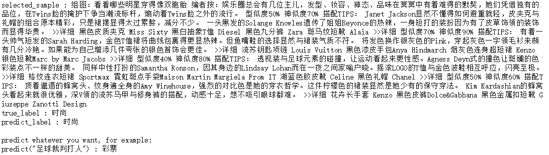

#Confusion Matrix
import numpy as np
import pandas as pd
from sklearn.metrics import confusion_matrix

def predictAll(test_X, batch_size=100):
    predict_value_list = []
    for i in range(0, len(test_X), batch_size):
        selected_X = test_X[i: i + batch_size]
        predict_value = session.run(predict_Y, {X_holder:selected_X})
        predict_value_list.extend(predict_value)
    return np.array(predict_value_list)

Y = predictAll(test_X)
y = np.argmax(Y, axis=1)
predict_label_list = labelEncoder.inverse_transform(y)
pd.DataFrame(confusion_matrix(test_label_list, predict_label_list), 
             columns=labelEncoder.classes_,
             index=labelEncoder.classes_ )

Run result: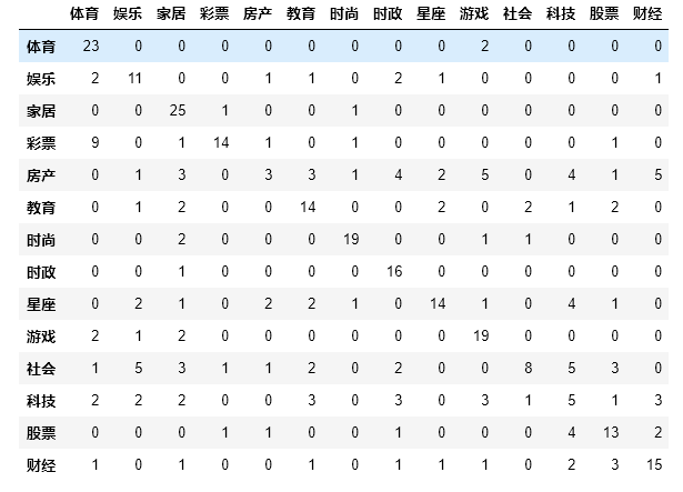

#Report Form
import numpy as np
from sklearn.metrics import precision_recall_fscore_support

def eval_model(y_true, y_pred, labels):
   # Calculate recision, Recall, f1, support for each classification
   p, r, f1, s = precision_recall_fscore_support(y_true, y_pred)
   # Calculate the average Precision, Recall, f1, support for the population
   tot_p = np.average(p, weights=s)
   tot_r = np.average(r, weights=s)
   tot_f1 = np.average(f1, weights=s)
   tot_s = np.sum(s)
   res1 = pd.DataFrame({
       u'Label': labels,
       u'Precision': p,
       u'Recall': r,
       u'F1': f1,
       u'Support': s
   })
   res2 = pd.DataFrame({
       u'Label': ['population'],
       u'Precision': [tot_p],
       u'Recall': [tot_r],
       u'F1': [tot_f1],
       u'Support': [tot_s]
   })
   res2.index = [999]
   res = pd.concat([res1, res2])
   return res[['Label', 'Precision', 'Recall', 'F1', 'Support']]

eval_model(test_label_list, predict_label_list, labelEncoder.classes_)

Run result: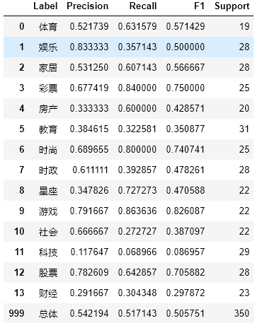

3. Sohu News Text Category (word2vec)

Create a new word2vec-based text categorization folder on your desktop. Enter cmd in the folder: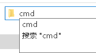


Create a new word2vec_test.ipynb: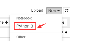

rename is: word2vec_test

There are two more files in the folder at this time: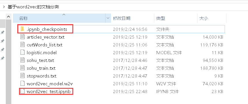

3.1 Data preparation

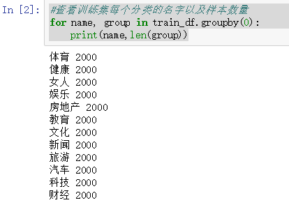
There are 24,000 samples in the training set, 12 classifications, and 2000 samples in each classification.
There are 12,000 samples in the test set, 12 classifications, and 1,000 samples in each classification.
Link: https://pan.baidu.com/s/1UbPjMpcp3kqvdd0HMAgMfQ Extraction Code: b53e
The file decompressed for the compressed package is shown in the red box below: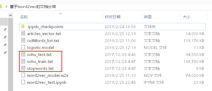

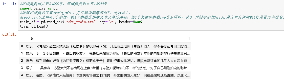
Load the training set into the variable train_df and print the first five lines of the training set, coded as follows:

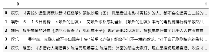
#There are 24,000 training set data and 12,000 test set data.
import pandas as pd
#Load the training set into the variable train_df and print the first five lines of the training set, coded as follows.
#There are three parameters in the read_csv method. The first parameter is the path to load the text file, the second key parameter sep is the separator, and the third key parameter header is whether the first line of the text file is the field name or not.
train_df = pd.read_csv('sohu_train.txt', sep='\t', header=None)
train_df.head()

#View the name of each category in the training set and the number of samples
for name, group in train_df.groupby(0):
    print(name,len(group))

#Load the test set and see the name of each category and the number of samples
test_df = pd.read_csv('sohu_test.txt', sep='\t', header=None)
for name, group in test_df.groupby(0):
    print(name, len(group))

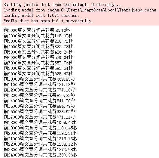
#Walk through 24,000 samples of the training set and use the cut method of the jieba library to get the word breaker list and assign it to the variable cutWords
#Determines whether a participle is a pause, or if it is not, adds it to the variable cutWords
import jieba
import time

train_df.columns = ['classification', 'Article']
stopword_list = [k.strip() for k in open('stopwords.txt', encoding='utf8').readlines() if k.strip() != '']
cutWords_list = []
i = 0
startTime = time.time()
for article in train_df['Article']:
 cutWords = [k for k in jieba.cut(article) if k not in stopword_list]
 i += 1
 if i % 1000 == 0:
     print('Front%d Total cost of article word breaking%.2f second' %(i, time.time()-startTime))
 cutWords_list.append(cutWords)

Run result: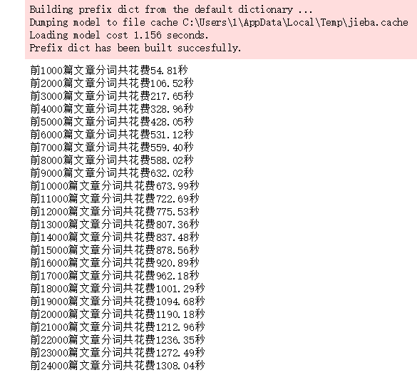

#Save word breaking results as local file cutWords_list.txt
with open('cutWords_list.txt', 'w') as file: 
    for cutWords in cutWords_list:
        file.write(' '.join(cutWords) + '\n')

The author provides links to text files that have been word-split: https://pan.baidu.com/s/1oKjLZjSkqE0LfLEvLxkBNw Extraction Code: oh3u

#Load word breaker file
with open('cutWords_list.txt') as file:
  cutWords_list = [k.split() for k in file.readlines()]

3.2 word 2vec model

To complete this step, you need to first install the gensim library, install the command: pip install gensim

#Invoke the LineSentence method in the gensim.models.word2vec library to instantiate the model object
from gensim.models import Word2Vec

word2vec_model = Word2Vec(cutWords_list, size=100, iter=10, min_count=20)

#Always prompt for warnings when invoking methods for model objects to avoid them
import warnings

warnings.filterwarnings('ignore')

#Call the wv.most_similar method of the Word2Vec model object to see words that have the closest meaning to photography.
#The wv.most_similar method has two parameters. The first parameter is the word to search for, and the second keyword parameter, topn, has a positive integer data type. It refers to how many most relevant words need to be listed. By default, it lists 10 most relevant words.
#The data type of the return value from the wv.most_similar method is a list, with each element in the list having a data type of tuple and two elements in the tuple, the first element having a related vocabulary, the second element having a degree of correlation and the data type floating point.
word2vec_model.wv.most_similar('Photography')

Run result: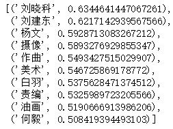

A simple example of using positive and negative as keyword parameters for the wv.most_similar method is to look at the results for women+men:

word2vec_model.most_similar(positive=['woman', 'Sir'], negative=['Man'], topn=1)

Run result: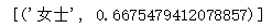

Look at the correlation between the two words as shown in the following figure: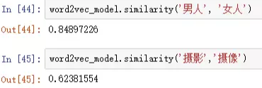

Save the Word2Vec model as a word2vec_model.w2v file with the following code:

word2vec_model.save('word2vec_model.w2v')

3.3 Feature Engineering:

#For each article, get the correlation vector of each participle in the word2vec model
#Then sum the correlation vectors of all the participles of an article in the word2vec model to get the average, that is, the correlation vectors of this article in the word2vec model
#When instantiating a Word2Vec object, the keyword parameter size is defined as 100, and the correlation matrix is 100 dimensions
#Defines the getVector function to get the word vector for each article, passing in two parameters, the first parameter is the result of article partitioning and the second parameter is the word2vec model object
#The variable vector_list derives the word vectors of all the participles in a single article through list derivation, converts them into ndarray objects by np.array method, and averages each column

#Method 1, general calculation with for loop
''''import numpy as np 
import time 

def getVector_v1(cutWords, word2vec_model):
    count = 0
    article_vector = np.zeros(word2vec_model.layer1_size)
    for cutWord in cutWords:
        if cutWord in word2vec_model:
            article_vector += word2vec_model[cutWord]
            count += 1
    return article_vector / count

startTime = time.time()
vector_list = []
i = 0
for cutWords in cutWords_list[:5000]:
    i += 1
    if i % 1000 ==0:
        print('Front%d Article Formation Word Vector Spending%.2f second' %(i, time.time()-startTime))
    vector_list.append(getVector_v1(cutWords, word2vec_model))
X = np.array(vector_list)

#The second method, calculated by mean s of pandas
''''import time 
import pandas as pd 

def getVector_v2(cutWords, word2vec_model):
    vector_list = [word2vec_model[k] for k in cutWords if k in word2vec_model]
    vector_df = pd.DataFrame(vector_list)
    cutWord_vector = vector_df.mean(axis=0).values
    return cutWord_vector

startTime = time.time()
vector_list = []
i = 0
for cutWords in cutWords_list[:5000]:
    i += 1
    if i % 1000 ==0:
        print('Front%d Article Formation Word Vector Spending%.2f second' %(i, time.time()-startTime))
    vector_list.append(getVector_v2(cutWords, word2vec_model))
X = np.array(vector_list)

#The third method, calculated by mean s of numpy
import time
import numpy as np

def getVector_v3(cutWords, word2vec_model):
    vector_list = [word2vec_model[k] for k in cutWords if k in word2vec_model]
    cutWord_vector = np.array(vector_list).mean(axis=0)
    return cutWord_vector

startTime = time.time()
vector_list = []
i = 0
for cutWords in cutWords_list:
    i += 1
    if i % 1000 ==0:
        print('Front%d Article Formation Word Vector Spending%.2f second' %(i, time.time()-startTime))
    vector_list.append(getVector_v3(cutWords, word2vec_model))
X = np.array(vector_list)

Run result: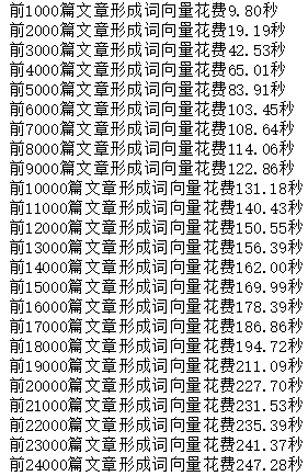

#Method 4, calculated by numpy add, divide
''''import time
import numpy as np

def getVector_v4(cutWords, word2vec_model):
    i = 0
    index2word_set = set(word2vec_model.wv.index2word)
    article_vector = np.zeros((word2vec_model.layer1_size))
    for cutWord in cutWords:
        if cutWord in index2word_set:
            article_vector = np.add(article_vector, word2vec_model.wv[cutWord])
            i += 1
    cutWord_vector = np.divide(article_vector, i)
    return cutWord_vector

startTime = time.time()
vector_list = []
i = 0
for cutWords in cutWords_list[:5000]:
    i += 1
    if i % 1000 ==0:
        print('Front%d Article Formation Word Vector Spending%.2f second' %(i, time.time()-startTime))
    vector_list.append(getVector_v4(cutWords, word2vec_model))
X = np.array(vector_list)

#Because it takes a long time to form the feature matrix, the feature matrix is saved as a file in order to avoid repeating the time in the future.
#Using the dump method of the ndarray object requires a parameter with a data type of string and a file name to save the file
X.dump('articles_vector.txt')

#Load the contents of this file to assign to variable X
X = np.load('articles_vector.txt')

3.4 Model training, model evaluation

3.4.1 Label Coding:

#Label Encoding
#Call the LabelEncoder method of sklearn.preprocessing library to label article categories
from sklearn.preprocessing import LabelEncoder
import pandas as pd

train_df = pd.read_csv('sohu_train.txt', sep='\t', header=None)
train_df.columns = ['classification', 'Article']
labelEncoder = LabelEncoder()
y = labelEncoder.fit_transform(train_df['classification'])

3.4.2 Logistic Regression Model

#Call the LogisticRegression method of the sklearn.linear_model library to instantiate the model object.
#Calling the train_test_split method of sklearn.model_selection library to partition training and test sets
from sklearn.linear_model import LogisticRegression
from sklearn.model_selection import train_test_split

train_X, test_X, train_y, test_y = train_test_split(X, y, test_size=0.2)
logistic_model = LogisticRegression()
logistic_model.fit(train_X, train_y)
logistic_model.score(test_X, test_y)

Run result:

3.4.3 Save Model

#Call the joblib method in the sklearn.externals library to save the model as a logistic.model file
from sklearn.externals import joblib

joblib.dump(logistic_model, 'logistic.model')

#Load Model
from sklearn.externals import joblib

logistic_model = joblib.load('logistic.model')

3.4.4 Cross-validation

#The results of cross-validation are more convincing.
#Call the ShuffleSplit method of the sklearn.model_selection library to instantiate the cross-validation object.
#Call the cross_val_score method of the sklearn.model_selection library to get a score for each cross-validation
from sklearn.linear_model import LogisticRegression
from sklearn.model_selection import ShuffleSplit
from sklearn.model_selection import cross_val_score

cv_split = ShuffleSplit(n_splits=5, train_size=0.7, test_size=0.2)
logistic_model = LogisticRegression()
score_ndarray = cross_val_score(logistic_model, X, y, cv=cv_split)
print(score_ndarray)
print(score_ndarray.mean())

Run result:

3.4.5 Model Test

#Model Test
#Call the load method of the joblib object in the sklearn.externals library to load the model assignment to the variable logistic_model.
#Call the pandas library read_csv method to read the test set data.
#Call the groupby method of the DataFrame object to group each category so that each article category is categorized accurately.
#Call the custom getVector method to convert the article to a correlation vector.
#Customize the getVectorMatrix method to get the characteristic matrix of the test set.
#Calling the transform method of the labelEncoder object labels the prediction label to get the prediction target value

import pandas as pd
import numpy as np
from sklearn.externals import joblib
import jieba 

def getVectorMatrix(article_series):
    return np.array([getVector_v3(jieba.cut(k), word2vec_model) for k in article_series])
    
logistic_model = joblib.load('logistic.model')
test_df = pd.read_csv('sohu_test.txt', sep='\t', header=None)
test_df.columns = ['classification', 'Article']
for name, group in test_df.groupby('classification'):
    featureMatrix = getVectorMatrix(group['Article'])
    target = labelEncoder.transform(group['classification'])
    print(name, logistic_model.score(featureMatrix, target))

Result of last code run:

3.5 Summary

word2vec model is applied. There are 24,000 training set data and 12,000 test set data.After cross-validation, the average model score is about 0.78.(In the validation effect of the test set, the seven categories of sports, education, health, culture, tourism, automobile and entertainment have higher scores, that is, they are easy to be classified correctly.The five categories of women, entertainment, news, science and technology, finance have low scores, which means they are difficult to classify correctly.)

4. Sohu News Text Category (TfidfVectorizer)

import pandas as pd

train_df = pd.read_csv('sohu_train.txt', sep='\t', header=None)
train_df.head()

for name, group in train_df.groupby(0):
    print(name,len(group))

Run result: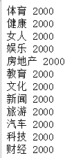

test_df = pd.read_csv('sohu_test.txt', sep='\t', header=None)
for name, group in test_df.groupby(0):
    print(name, len(group))

Run result: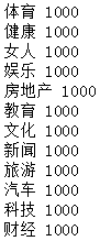

with open('stopwords.txt', encoding='utf8') as file:
  stopWord_list = [k.strip() for k in file.readlines()]

Run result: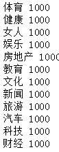

with open('stopwords.txt', encoding='utf8') as file:
  stopWord_list = [k.strip() for k in file.readlines()]

import jieba
import time

train_df.columns = ['classification', 'Article']
stopword_list = [k.strip() for k in open('stopwords.txt', encoding='utf8').readlines() if k.strip() != '']
cutWords_list = []
i = 0
startTime = time.time()
for article in train_df['Article']:
   cutWords = [k for k in jieba.cut(article) if k not in stopword_list]
   i += 1
   if i % 1000 == 0:
       print('Front%d Total cost of article word breaking%.2f second' %(i, time.time()-startTime))
   cutWords_list.append(cutWords) 

with open('cutWords_list.txt', 'w') as file: 
    for cutWords in cutWords_list:
        file.write(' '.join(cutWords) + '\n')

with open('cutWords_list.txt') as file:
    cutWords_list = [k.split() for k in file.readlines()]

#Feature Engineering
X = tfidf.fit_transform(train_df[1])
print('Glossary size:', len(tfidf.vocabulary_))
print(X.shape)

Run result: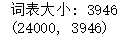

#Call the LabelEncoder method of the sklearn.preprocessing library to label the article categories.
#The last line of code looks at the shape of the prediction target.

from sklearn.preprocessing import LabelEncoder
import pandas as pd

train_df = pd.read_csv('sohu_train.txt', sep='\t', header=None)
labelEncoder = LabelEncoder()
y = labelEncoder.fit_transform(train_df[0])
y.shape

Run result:

#Call the LogisticRegression method of the sklearn.linear_model library to instantiate the model object.
#Call the train_test_split method of the sklearn.model_selection library to divide the training and test sets.

from sklearn.linear_model import LogisticRegression
from sklearn.model_selection import train_test_split

train_X, test_X, train_y, test_y = train_test_split(X, y, test_size=0.2)
logistic_model = LogisticRegression(multi_class='multinomial', solver='lbfgs')
logistic_model.fit(train_X, train_y)
logistic_model.score(test_X, test_y)

Run result: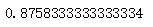

#To save the model, you need to install the pickle library first. Install the command: pip install pickle
#Calling the dump method of the pickle library to save the model requires two parameters.
#The first parameter is a saved object and can be of any data type, since there are three models to save, the first parameter in the code below is a dictionary.
#The second parameter is the saved file object, with a data type of _io.BufferedWriter

import pickle

with open('tfidf.model', 'wb') as file:
    save = {
        'labelEncoder' : labelEncoder,
        'tfidfVectorizer' : tfidf,
        'logistic_model' : logistic_model
    }
    pickle.dump(save, file)

#Call the load method of the pickle library to load the saved model object
import pickle

with open('tfidf.model', 'rb') as file:
    tfidf_model = pickle.load(file)
    tfidfVectorizer = tfidf_model['tfidfVectorizer']
    labelEncoder = tfidf_model['labelEncoder']
    logistic_model = tfidf_model['logistic_model']

#Call the pandas read_csv method to load the training set data.
#The transform ation method of the TfidfVectorizer object is called to obtain the feature matrix.
#Call the transform method of the LabelEncoder object to get the predicted target value.

import pandas as pd

train_df = pd.read_csv('sohu_train.txt', sep='\t', header=None)
X = tfidfVectorizer.transform(train_df[1])
y = labelEncoder.transform(train_df[0])
```python
#The Logistic Regression model object is instantiated by calling the LogisticRegression method of the sklearn.linear_model library.
#Call the ShuffleSplit method of the sklearn.model_selection library to instantiate the cross-validation object.
#Call the cross_val_score method of the sklearn.model_selection library to get the score for each cross-validation.
#Final print each score and average score

from sklearn.linear_model import LogisticRegression
from sklearn.model_selection import ShuffleSplit
from sklearn.model_selection import cross_val_score

logistic_model = LogisticRegression(multi_class='multinomial', solver='lbfgs')
cv_split = ShuffleSplit(n_splits=5, test_size=0.3)
score_ndarray = cross_val_score(logistic_model, X, y, cv=cv_split)
print(score_ndarray)
print(score_ndarray.mean())

Run result:

#Draw confusion matrix
from sklearn.model_selection import train_test_split
from sklearn.linear_model import LogisticRegressionCV
from sklearn.metrics import confusion_matrix
import pandas as pd

train_X, test_X, train_y, test_y = train_test_split(X, y, test_size=0.2)
logistic_model = LogisticRegressionCV(multi_class='multinomial', solver='lbfgs')
logistic_model.fit(train_X, train_y)
predict_y = logistic_model.predict(test_X)
pd.DataFrame(confusion_matrix(test_y, predict_y), 
             columns=labelEncoder.classes_, 
             index=labelEncoder.classes_)

Run result: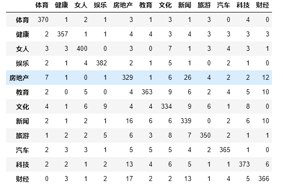

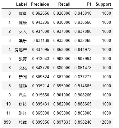
#Draw precision, recall, f1-score, support report tables
import numpy as np
from sklearn.metrics import precision_recall_fscore_support

def eval_model(y_true, y_pred, labels):
    # Calculate recision, Recall, f1, support for each classification
    p, r, f1, s = precision_recall_fscore_support(y_true, y_pred)
    # Calculate the average Precision, Recall, f1, support for the population
    tot_p = np.average(p, weights=s)
    tot_r = np.average(r, weights=s)
    tot_f1 = np.average(f1, weights=s)
    tot_s = np.sum(s)
    res1 = pd.DataFrame({
        u'Label': labels,
        u'Precision': p,
        u'Recall': r,
        u'F1': f1,
        u'Support': s
    })
    res2 = pd.DataFrame({
        u'Label': ['population'],
        u'Precision': [tot_p],
        u'Recall': [tot_r],
        u'F1': [tot_f1],
        u'Support': [tot_s]
    })
    res2.index = [999]
    res = pd.concat([res1, res2])
    return res[['Label', 'Precision', 'Recall', 'F1', 'Support']]

predict_y = logistic_model.predict(test_X)
eval_model(test_y, predict_y, labelEncoder.classes_)

Run result: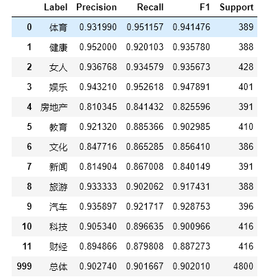

#Model testing is the prediction of a completely new set of tests.
#Call the read_csv method of the pandas library to read the test set file.
#The transform ation method of the TfidfVectorizer object is called to obtain the feature matrix.
#Call the transform ation method of the LabelEncoder object to get the predicted target value

import pandas as pd

test_df = pd.read_csv('sohu_test.txt', sep='\t', header=None)
test_X = tfidfVectorizer.transform(test_df[1])
test_y = labelEncoder.transform(test_df[0])
predict_y = logistic_model.predict(test_X)
eval_model(test_y, predict_y, labelEncoder.classes_)

Run result: