introduction
Transformer is the basic structure of almost all pre training models today. Maybe we usually pay more attention to how to make better use of the trained GPT, BERT and other models for fine tune, but equally important, we need to know how to build these powerful models. Therefore, in this paper, we mainly study how to implement it in code under the PyTorch framework "Attention is All You Need" The structure of the original Transformer in the paper.
1, Preparatory work
The test environment for this article is Python 3.6 + and PyTorch 1.6
import numpy as np
import torch
import torch.nn as nn
import torch.nn.functional as F
import math, copy, time
import matplotlib.pyplot as plt
import seaborn
seaborn.set_context(context="talk")
%matplotlib inline
2, Background introduction
when talking about sequence modeling, we first think of RNN and its variants, but the disadvantage of RNN model is also very obvious: it needs sequential calculation, so it is difficult to parallel. Therefore, network models such as Extended Neural GPU, ByteNet and ConvS2S appear. These models are based on CNN, which is easy to parallel, but compared with RNN, it is difficult to learn long-distance dependencies.
the Transformer in this paper uses the self attention mechanism, which can pay attention to the whole sentence when encoding each word, so as to solve the problem of long-distance dependence. At the same time, the calculation of self attention can use matrix multiplication to calculate all times at once, so it can make full use of computing resources.
Three, model structure
1. Encoder decoder structure
the sequence conversion model is based on the encoder decoder structure. The so-called sequence conversion model is to convert an input sequence into another output sequence, and their lengths are likely to be different. For example, in machine translation based on neural network, the input is French sentences and the output is English sentences, which is a sequence transformation model. Similar problems, including text summarization and dialogue, can be regarded as sequence transformation problems. We mainly focus on machine translation here, but any problem where the input is a sequence and the output is another sequence can consider using the encoder decoder structure.
Encoder will input the sequence
(
x
1
,
.
.
,
x
n
)
(x_1,..,x_n)
(x1,..., xn) is encoded into a continuous sequence
z
=
(
z
1
,
.
.
,
z
n
)
z=(z_1,..,z_n)
z=(z1,..,zn). And the Decoder
z
z
z to decode the output sequence
y
=
(
y
1
,
.
.
,
y
m
)
y=(y_1,..,y_m)
y=(y1,..,ym). The Decoder is auto regressive. It takes the output of the previous time as the input of the current time. The codes corresponding to the encoder Decoder structure are as follows:
class EncoderDecoder(nn.Module):
    """
    A standard Encoder-Decoder architecture. Base for this and many other models.
    take encoder The last one Block Separately to decoder Each of block,then decoder Output generation.
    """

    def __init__(self, encoder, decoder, src_embed, tgt_embed, generator):
        super(EncoderDecoder, self).__init__()
        self.encoder = encoder
        self.decoder = decoder
        self.src_embed = src_embed
        self.tgt_embed = tgt_embed
        self.generator = generator

    def forward(self, src, tgt, src_mask, tgt_mask):
        """
        Take in and process masked src and target sequences.
        """
        return self.decode(self.encode(src, src_mask), src_mask, tgt, tgt_mask)

    def encode(self, src, src_mask):
        return self.encoder(self.src_embed(src), src_mask)

    def decode(self, memory, src_mask, tgt, tgt_mask):
        return self.decoder(self.tgt_embed(tgt), memory, src_mask, tgt_mask)
class Generator(nn.Module):
    """
    Define standard linear + softmax generation step.
    Map to vocab Dimension and do softmax Get the probability of generating each word
    """

    def __init__(self, d_model, vocab):
        super(Generator, self).__init__()
        self.proj = nn.Linear(d_model, vocab)

    def forward(self, x):
        return F.log_softmax(self.proj(x), dim=-1)
encoder decoder defines a general encoder decoder architecture, including encoder, decoder and src_embed,target_ Both embedded and generator are arguments passed in by the constructor. In this way, it will be more convenient for us to experiment and replace different components.
Explain the meaning of various parameters: encoder and encoder represent encoder and decoder respectively; src_embed,tgt_ Embedded represents the method of encoding the ID sequences of the source language and the target language into word vectors respectively; The generator outputs the words at the current time according to the implicit state of the decoder at the current time. The specific implementation method (i.e. generator class) has been given above.
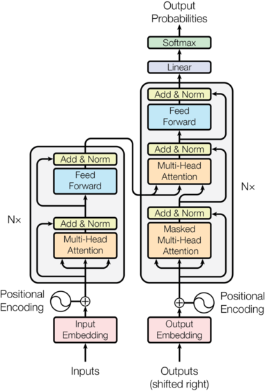
The Transformer model also follows the Encoder Decoder architecture. Its Encoder is composed of N=6 identical encoderlayers, and each EncoderLayer contains a self attention sublayer layer and a feed forward sublayer layer; Its Decoder is also composed of N=6 identical decoderlayers. Each DecoderLayer includes a self attention sublayer layer, an Encoder Decoder attention sublayer layer and a feed forward sublayer layer. The overall architecture of Transformer is shown below:
2.Encoder and Decoder Stacks
2.1 Encoder
as mentioned earlier, the Encoder is stacked by N=6 encoderlayers with the same structure, so the code for defining the Encoder is as follows:
def clones(module, N):
    """
    Produce N identical layers.
    """
    return nn.ModuleList([copy.deepcopy(module) for _ in range(N)])
class Encoder(nn.Module):
    """
    Core encoder is a stack of N layers.
    """

    def __init__(self, layer, N):
        super(Encoder, self).__init__()
        self.layers = clones(layer, N)
        self.norm = LayerNorm(layer.size)

    def forward(self, x, mask):
        """
        Pass the input (and mask) through each layer in turn.
        """
        for layer in self.layers:
            x = layer(x, mask)
        return self.norm(x)
That is, the Encoder will make a deep copy of the incoming layer N times, then let the incoming Tensor pass through the N layers in turn, and finally through a layer of Layer Normalization.
class LayerNorm(nn.Module):
    """
    Construct a layernorm module, see https://arxiv.org/abs/1607.06450 for details.
    """

    def __init__(self, features, eps=1e-6):
        super(LayerNorm, self).__init__()
        self.a_2 = nn.Parameter(torch.ones(features))
        self.b_2 = nn.Parameter(torch.zeros(features))
        self.eps = eps

    def forward(self, x):
        mean = x.mean(-1, keepdim=True)
        std = x.std(-1, keepdim=True)
        return self.a_2 * (x - mean) / (std + self.eps) + self.b_2
According to the original paper, the output of each sub layer of each encoder layer should be
L
a
y
e
r
N
o
r
m
(
x
+
S
u
b
l
a
y
e
r
(
x
)
)
LayerNorm(x+Sublayer(x))
LayerNorm(x+Sublayer(x)), where Sublayer(x) is an abstract function implemented for the sublayer structure. Some modifications have been made here. First, a Dropout layer is added after the output of each sub layer. The other difference is to put the LayerNorm layer in front. That is, the actual output of each sublayer is:
x
+
D
r
o
p
o
u
t
(
S
u
b
l
a
y
e
r
(
L
a
y
e
r
N
o
r
m
(
x
)
)
)
x+Dropout(Sublayer(LayerNorm(x)))
x+Dropout(Sublayer(LayerNorm(x)))
In order to speed up the residual connection, all sub layers in the model, including the Embedding layer, set their output dimensions to
d
m
o
d
e
l
=
512
d_{model}=512
dmodel=512. So we have the following code:
class SublayerConnection(nn.Module):
    """
    A residual connection followed by a layer norm.
    Note for code simplicity the norm is first as opposed to last.
    """

    def __init__(self, size, dropout):
        super(SublayerConnection, self).__init__()
        self.norm = LayerNorm(size)
        self.dropout = nn.Dropout(dropout)

    def forward(self, x, sublayer):
        """
        Apply residual connection to any sublayer with the same size.
        """
        return x + self.dropout(sublayer(self.norm(x)))
As mentioned above, EncoderLayer is composed of two sub layers: self attention and feed forward, so the following code is available:
class EncoderLayer(nn.Module):
    """
    Encoder is made up of self-attn and feed forward.
    """

    def __init__(self, size, self_attn, feed_forward, dropout):
        super(EncoderLayer, self).__init__()
        self.self_attn = self_attn
        self.feed_forward = feed_forward
        self.sublayer = clones(SublayerConnection(size, dropout), 2)
        self.size = size

    def forward(self, x, mask):
        x = self.sublayer[0](x, lambda x: self.self_attn(x, x, x, mask))
        return self.sublayer[1](x, self.feed_forward)
2.2 decoder
Decoder is also provided by N = 6 N=6 N=6 decoderlayers with the same structure are stacked.
class Decoder(nn.Module):
    """
    Generic N layer decoder with masking.
    """

    def __init__(self, layer, N):
        super(Decoder, self).__init__()
        self.layers = clones(layer, N)
        self.norm = LayerNorm(layer.size)

    def forward(self, x, memory, src_mask, tgt_mask):
        for layer in self.layers:
            x = layer(x, memory, src_mask, tgt_mask)
        return self.norm(x)
As mentioned earlier, in addition to two sub layers like the Encoder layer, a decoder layer also has an Encoder decoder attention sub layer. This sub layer allows the model to consider the output of the last layer of Encoder at all times during decoding.
class DecoderLayer(nn.Module):
    """
    Decoder is made of self-attn, src-attn, and feed forward.
    """

    def __init__(self, size, self_attn, src_attn, feed_forward, dropout):
        super(DecoderLayer, self).__init__()
        self.size = size
        self.self_attn = self_attn
        self.src_attn = src_attn
        self.feed_forward = feed_forward
        self.sublayer = clones(SublayerConnection(size, dropout), 3)

    def forward(self, x, memory, src_mask, tgt_mask):
        m = memory
        x = self.sublayer[0](x, lambda x: self.self_attn(x, x, x, tgt_mask))
        x = self.sublayer[1](x, lambda x: self.src_attn(x, m, m, src_mask))
        return self.sublayer[2](x, self.feed_forward)
The extra Attention sublayer (SRC in the code)_ The implementation of Attn) is the same as self Attention, except Src_ The Query of Attn comes from the output of the previous layer Decoder, but the Key and Value come from the output of the last layer of Encoder (memory in the code); The Q, K and V of self Attention are all from the output of the previous layer.
there is another key difference between Decoder and Encoder: when decoding the t-th time, the Decoder can only use the input less than t time, but cannot use the input at t+1 time and after. Therefore, we need a function to generate a Mask matrix:
def subsequent_mask(size):
    """
    Mask out subsequent positions.
    """
    attn_shape = (1, size, size)
    subsequent_mask = np.triu(np.ones(attn_shape), k=1).astype('uint8')
    return torch.from_numpy(subsequent_mask) == 0
The above code means to use the triu function to generate an upper triangular matrix, and then use matrix == 0 to get the required lower triangular matrix. All upper triangles are 0 and all lower triangles are 1.
plt.figure(figsize=(5,5))
plt.imshow(subsequent_mask(20)[0])
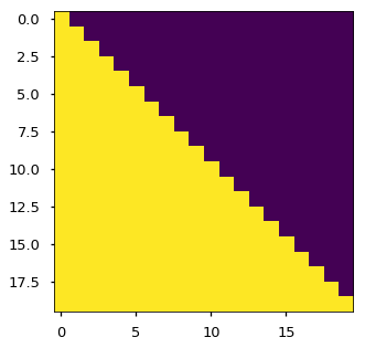
Thus, when training, you can only see the front information, not all the information.
3.Attention
3.1self-attention
attention (including self attention and ordinary Attention) can be regarded as a function. Its input is Query,Key and Value, and its output is Tensor. The output is the weighted average of Value, and the weight comes from the calculation of Query and Key.
the paper first mentioned the scaled dot product attention, as shown in the following figure:
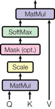
The specific calculation is to dot multiply a group of queries and all keys, and then divide by
d
k
\sqrt{d_k}
dk
Ensure the stability of subsequent gradients, then normalize these scores by softmax as the similarity between query and Keys, that is, the weight of the weighted average of values, and finally make the weighted average of all values as the output. Here, it is directly expressed by matrix:
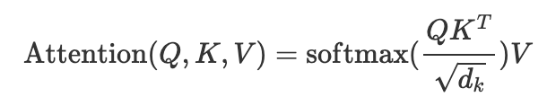
The code is as follows:
def attention(query, key, value, mask=None, dropout=None):
    """
    Compute 'Scaled Dot Product Attention'
    """
    d_k = query.size(-1)
    scores = torch.matmul(query, key.transpose(-2, -1)) / math.sqrt(d_k)
    # Give the padding part a small value
    if mask is not None:
        scores = scores.masked_fill(mask == 0, -1e9)
    # Normalized to obtain attention weight
    p_attn = F.softmax(scores, dim=-1)
    # dropout
    if dropout is not None:
        p_attn = dropout(p_attn)
    # Returns the weighted vector and attention weight
    return torch.matmul(p_attn, value), p_attn
3.2 Multi-Head Attention
the most important multi head attention in this paper is based on scaled dot product attention. In fact, it is very simple. The previously defined group of Q, K and V can make a word attach to related words. We can define multiple groups of Q, K and V, which can focus on different contexts:

From the above figure, we can get the following calculation formula:
M
u
l
t
i
H
e
a
d
(
Q
,
K
,
V
)
=
C
o
n
c
a
t
(
h
e
a
d
1
,
.
.
.
,
h
e
a
d
h
)
W
O
h
e
a
d
i
=
A
t
t
e
n
t
i
o
n
(
Q
W
i
Q
,
K
W
i
K
,
V
W
i
V
)
MultiHead(Q,K,V)=Concat(head_1,...,head_h)W^O\\head_i=Attention(QW^Q_i,KW^K_i,VW^V_i)
MultiHead(Q,K,V)=Concat(head1,...,headh)WOheadi=Attention(QWiQ,KWiK,VWiV)
Used in the paper
h
=
8
h=8
h=8 heads, so at this time
d
k
=
d
v
=
d
m
o
d
e
l
/
h
=
64
d_k=d_v=d_{model}/h=64
dk=dv=dmodel/h=64. Although the number of heads is increased by 8 times, the overall calculation cost is basically unchanged because the dimension of each Head is reduced by 8 times.
the code of multi head attention is as follows:
class MultiHeadedAttention(nn.Module):
    """
    Implements 'Multi-Head Attention' proposed in the paper.
    """

    def __init__(self, h, d_model, dropout=0.1):
        """
        Take in model size and number of heads.
        """
        super(MultiHeadedAttention, self).__init__()
        assert d_model % h == 0
        # We assume d_v always equals d_k
        self.d_k = d_model // h
        self.h = h
        self.linears = clones(nn.Linear(d_model, d_model), 4)
        self.attn = None
        self.dropout = nn.Dropout(p=dropout)

    def forward(self, query, key, value, mask=None):
        if mask is not None:
            # Same mask applied to all h heads.
            mask = mask.unsqueeze(1)
        nbatches = query.size(0)

        # 1) Do all the linear projections in batch from d_model => h x d_k
        query, key, value = [l(x).view(nbatches, -1, self.h, self.d_k).transpose(1, 2)
                             for l, x in zip(self.linears, (query, key, value))]

        # 2) Apply attention on all the projected vectors in batch.
        x, self.attn = attention(query, key, value, mask=mask, dropout=self.dropout)

        # 3) "Concat" using a view and apply a final linear.
        x = x.transpose(1, 2).contiguous().view(nbatches, -1, self.h * self.d_k)
        return self.linears[-1](x)
3.3 application of attention in model
in Transformer, multi head attention is used in three places:
- Encoder Decoder Attention layer of Decoder. query comes from the output of the previous layer Decoder, while key and value come from the output of the last layer encoder. This Attention layer makes the Decoder consider the output of the last layer encoder at all times during decoding. It is a common Attention mechanism in encoder Decoder architecture.
- Self attention layer of Encoder. query, key and value all come from the same place, that is, the output of the previous layer Encoder.
- The self attention layer of the Decoder. query, key and value all come from the same place, that is, the output of the previous layer Decoder, but the Mask makes it unable to access the output of the future time.
4.Feed-Forward
in addition to the Attention sublayer, each layer of Encoder and Decoder also includes a feed forward sublayer, that is, the full connection layer. The full connection layer at each time can be calculated independently and in parallel (of course, the parameters are shared). The full connection layer consists of two linear transformations and ReLU activation between them:
F
F
N
(
x
)
=
m
a
x
(
0
,
x
W
1
+
b
1
)
W
2
+
b
2
FFN(x)=max(0,xW_1+b_1)W_2+b_2
FFN(x)=max(0,xW1+b1)W2+b2
The input and output of the full connection layer are
d
m
o
d
l
e
=
512
d_{modle}=512
dmodle = 512 dimensional, and the number of intermediate hidden units is
d
f
f
=
2048
d_ff=2048
dff=2048. The code implementation is very simple:
class PositionwiseFeedForward(nn.Module):
    """
    Implements FFN equation.
    """

    def __init__(self, d_model, d_ff, dropout=0.1):
        super(PositionwiseFeedForward, self).__init__()
        self.w_1 = nn.Linear(d_model, d_ff)
        self.w_2 = nn.Linear(d_ff, d_model)
        self.dropout = nn.Dropout(dropout)

    def forward(self, x):
        return self.w_2(self.dropout(F.relu(self.w_1(x))))
5.Embeddings
like most NLP tasks, the input word sequence is an ID sequence, so there needs to be an Embeddings layer.
class Embeddings(nn.Module):
    def __init__(self, d_model, vocab):
        super(Embeddings, self).__init__()
        # lut => lookup table
        self.lut = nn.Embedding(vocab, d_model)
        self.d_model = d_model

    def forward(self, x):
        return self.lut(x) * math.sqrt(self.d_model)
It should be noted that in the Embeddings layer, all weights are expanded d m o d e l \sqrt{d_{model}} dmodel Times
5.1 Positional Encoding
Transformer does not consider the order (position) relationship of words. In order to solve this problem, positional encoding is introduced. The formula used in the paper is as follows:
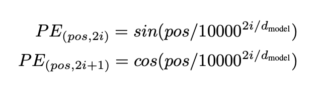
p
o
s
pos
pos means where in this sentence,
i
i
i represents the dimension of embedding. Therefore, the value of each dimension of each position of this sentence can be calculated through trigonometric function.
For example, if the length of the input ID sequence is 10, the size of Tensor after passing through the Embeddings layer is (10512), and the range of pos in the above formula is 0-9; For different dimensions, the range here is 0-511. sin function is used for even dimension and cos function is used for odd dimension.
The advantages of this location coding are: P E p o s + k PE_{pos+k} PEpos+k , can be expressed as P E p o s PE_{pos} PEpos linear function, so that the network can easily learn the relationship between relative positions. The location code is as follows:
class PositionalEncoding(nn.Module):
    """
    Implement the PE function.
    """

    def __init__(self, d_model, dropout, max_len=5000):
        super(PositionalEncoding, self).__init__()
        self.dropout = nn.Dropout(p=dropout)

        # Compute the positional encodings once in log space.
        pe = torch.zeros(max_len, d_model)
        position = torch.arange(0, max_len).unsqueeze(1)
        div_term = torch.exp(torch.arange(0, d_model, 2) * -(math.log(10000.0) / d_model))
        pe[:, 0::2] = torch.sin(position * div_term)
        pe[:, 1::2] = torch.cos(position * div_term)
        pe = pe.unsqueeze(0)
        self.register_buffer('pe', pe)

    def forward(self, x):
        x = x + self.pe[:, :x.size(1)]
        return self.dropout(x)
6. Complete model
here we define a function. The input is a hyperparameter and the output is a model built according to the hyperparameter:
def make_model(src_vocab, tgt_vocab, N=6, d_model=512, d_ff=2048, h=8, dropout=0.1):
    """
    Helper: Construct a model from hyperparameters.
    """
    c = copy.deepcopy
    attn = MultiHeadedAttention(h, d_model)
    ff = PositionwiseFeedForward(d_model, d_ff, dropout)
    position = PositionalEncoding(d_model, dropout)
    model = EncoderDecoder(
        Encoder(EncoderLayer(d_model, c(attn), c(ff), dropout), N),
        Decoder(DecoderLayer(d_model, c(attn), c(attn), c(ff), dropout), N),
        nn.Sequential(Embeddings(d_model, src_vocab), c(position)),
        nn.Sequential(Embeddings(d_model, tgt_vocab), c(position)),
        Generator(d_model, tgt_vocab))

    # This was important from their code.
    # Initialize parameters with Glorot / fan_avg.
    for p in model.parameters():
        if p.dim() > 1:
        	# initialization
            nn.init.xavier_uniform_(p)
    return model
4, Model training
first, we need a Batch class to provide Batch data and construct the required mask:
class Batch(object):
    """
    Object for holding a batch of data with mask during training.
    """

    def __init__(self, src, trg=None, pad=0):
        self.src = src
        self.src_mask = (src != pad).unsqueeze(-2)
        if trg is not None:
            self.trg = trg[:, :-1]
            self.trg_y = trg[:, 1:]
            self.trg_mask = self.make_std_mask(self.trg, pad)
            self.ntokens = (self.trg_y != pad).sum().item()

    @staticmethod
    def make_std_mask(tgt, pad):
        """
        Create a mask to hide padding and future words.
        """
        tgt_mask = (tgt != pad).unsqueeze(-2)
        tgt_mask = tgt_mask & subsequent_mask(tgt.size(-1))
        return tgt_mask
It is worth noting that the mask in the decoding phase (TRG in the code)_ Mask) needs to mask the output of the future time, which has implemented the corresponding function (i.e. subsequence) earlier_ Mask function).
next, write the training code for running an epoch, which is very simple:
def run_epoch(data_iter, model, loss_compute):
    """
    Standard Training and Logging Function
    """
    start = time.time()
    total_tokens = 0
    total_loss = 0
    tokens = 0
    for i, batch in enumerate(data_iter):
        out = model.forward(batch.src, batch.trg, batch.src_mask, batch.trg_mask)
        loss = loss_compute(out, batch.trg_y, batch.ntokens)
        total_loss += loss
        total_tokens += batch.ntokens
        tokens += batch.ntokens
        if i % 50 == 1:
            elapsed = time.time() - start
            print("Epoch Step: %d Loss: %f Tokens per Sec: %f" % (i, loss / batch.ntokens, tokens / elapsed))
            start = time.time()
            tokens = 0
    return total_loss / total_tokens
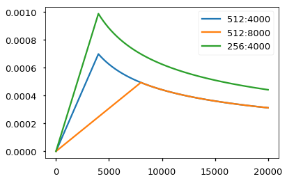
for the optimizer, the paper selects the common Adam optimizer, and the corresponding optimizer parameters are β 1 = 0.9 , β 2 = 0.98 , ϵ = 1 0 − 9 \beta_1=0.9,\beta_2=0.98,\epsilon=10^-9 β 1=0.9, β 2=0.98, ϵ= 10−9. In particular, the more important learning rate parameters change dynamically with the progress of training, that is, at the beginning w a r m u p s t e p s warmup_steps In warmups teps step, the learning rate increases linearly; Then slowly reduce the nonlinearity. In the paper w a r m u p s t e p s = 4000 warmup_steps=4000 warmupsteps=4000
class NoamOpt(object):
    """
    Optim wrapper that implements rate.
    """

    def __init__(self, model_size, factor, warmup, optimizer):
        self.optimizer = optimizer
        self._step = 0
        self.warmup = warmup
        self.factor = factor
        self.model_size = model_size
        self._rate = 0

    def step(self):
        """
        Update parameters and rate.
        """
        self._step += 1
        rate = self.rate()
        for p in self.optimizer.param_groups:
            p['lr'] = rate
        self._rate = rate
        self.optimizer.step()

    def rate(self, step=None):
        if step is None:
            step = self._step
        return self.factor * (self.model_size ** (-0.5) * min(step ** (-0.5), step * self.warmup ** (-1.5)))


def get_std_opt(model):
    return NoamOpt(model.src_embed[0].d_model, 2, 4000,
                   torch.optim.Adam(model.parameters(), lr=0, betas=(0.9, 0.98), eps=1e-9))
# Three settings of the lrate hyperparameters.
opts = [NoamOpt(512, 1, 4000, None),
        NoamOpt(512, 1, 8000, None),
        NoamOpt(256, 1, 4000, None)]
plt.plot(np.arange(1, 20000), [[opt.rate(i) for opt in opts] for i in range(1, 20000)])
plt.legend(["512:4000", "512:8000", "256:4000"])
three kinds of Regularization are used in the paper, one is Dropout and the other is residual connection, which have been explained earlier. The last one is Label Smoothing. Although Label Smoothing increases the confusion of model training, it does increase the accuracy and BLEU. The specific implementation is as follows:
class LabelSmoothing(nn.Module):
    """
    Implement label smoothing.
    """

    def __init__(self, size, padding_idx, smoothing=0.0):
        super(LabelSmoothing, self).__init__()
        self.criterion = nn.KLDivLoss(reduction='sum')
        self.padding_idx = padding_idx
        self.confidence = 1.0 - smoothing
        self.smoothing = smoothing
        self.size = size
        self.true_dist = None

    def forward(self, x, target):
        assert x.size(1) == self.size
        true_dist = x.clone()
        true_dist.fill_(self.smoothing / (self.size - 2))
        true_dist.scatter_(1, target.unsqueeze(1), self.confidence)
        true_dist[:, self.padding_idx] = 0
        mask = torch.nonzero(target == self.padding_idx)
        if mask.size(0) > 0:
            true_dist.index_fill_(0, mask.squeeze(), 0.0)
        self.true_dist = true_dist
        return self.criterion(x, true_dist)
5, Example
the task to be completed in the paper is a machine translation task, but it may be a little troublesome, so let's complete a simple replication task to test our model, that is, given the token sequence from a small vocabulary, our goal is to generate the same token sequence through the encoder decoder structure, for example, the input is [1,2,3,4,5], Then the generated sequence should also be [1,2,3,4,5].
the task data generation code is as follows, let src=trg.
def data_gen(V, batch, nbatches):
    """
    Generate random data for a src-tgt copy task.
    """
    for i in range(nbatches):
        data = torch.from_numpy(np.random.randint(1, V, size=(batch, 10)))
        data[:, 0] = 1
        yield Batch(src=data, trg=data, pad=0)
Then there is a method to calculate loss:
class SimpleLossCompute(object):
    """
    A simple loss compute and train function.
    """

    def __init__(self, generator, criterion, opt=None):
        self.generator = generator
        self.criterion = criterion
        self.opt = opt

    def __call__(self, x, y, norm):
        x = self.generator(x)
        loss = self.criterion(x.contiguous().view(-1, x.size(-1)), y.contiguous().view(-1)) / norm
        loss.backward()
        if self.opt is not None:
            self.opt.step()
            self.opt.optimizer.zero_grad()
        return loss.item() * norm
In the prediction stage, it is an autoregressive model. For simplicity, we directly use greedy search (generally Beam Search), that is, the word with the greatest probability is taken as the output at each time.
def greedy_decode(model, src, src_mask, max_len, start_symbol):
    memory = model.encode(src, src_mask)
    ys = torch.ones(1, 1, dtype=torch.long).fill_(start_symbol)
    for i in range(max_len - 1):
        out = model.decode(memory, src_mask, ys, subsequent_mask(ys.size(1)))
        prob = model.generator(out[:, -1])
        # Select the output with the highest probability
        _, next_word = torch.max(prob, dim=1)
        # Get the next word
        next_word = next_word.item()
        # Splicing
        ys = torch.cat([ys, torch.ones(1, 1, dtype=torch.long).fill_(next_word)], dim=1)
    return ys
Finally, running this example, we can see that Transformer has been able to complete the replication task perfectly in a few minutes!
# Train the simple copy task.
V = 11
# Label smoothing
criterion = LabelSmoothing(size=V, padding_idx=0, smoothing=0.0)
# Construction model
model = make_model(V, V, N=2)
# Model optimizer
model_opt = NoamOpt(model.src_embed[0].d_model, 1, 400,
                    torch.optim.Adam(model.parameters(), lr=0, betas=(0.9, 0.98), eps=1e-9))

# 15 rounds of training verification
for epoch in range(15):
    model.train()
    run_epoch(data_gen(V, 30, 20), model, SimpleLossCompute(model.generator, criterion, model_opt))
    model.eval()
    print(run_epoch(data_gen(V, 30, 5), model, SimpleLossCompute(model.generator, criterion, None)))

# This code predicts a translation using greedy decoding for simplicity.
print()
print("{}predict{}".format('*' * 10, '*' * 10))
# forecast
model.eval()
src = torch.tensor([[1, 2, 3, 4, 5, 6, 7, 8, 9, 10]])
src_mask = torch.ones(1, 1, 10)
print(greedy_decode(model, src, src_mask, max_len=10, start_symbol=1))
Epoch Step: 1 Loss: 3.023465 Tokens per Sec: 403.074173
Epoch Step: 1 Loss: 1.920030 Tokens per Sec: 641.689380
1.9274832487106324
Epoch Step: 1 Loss: 1.940011 Tokens per Sec: 432.003378
Epoch Step: 1 Loss: 1.699767 Tokens per Sec: 641.979665
1.657595729827881
Epoch Step: 1 Loss: 1.860276 Tokens per Sec: 433.320240
Epoch Step: 1 Loss: 1.546011 Tokens per Sec: 640.537198
1.4888023376464843
Epoch Step: 1 Loss: 1.682198 Tokens per Sec: 432.092305
Epoch Step: 1 Loss: 1.313169 Tokens per Sec: 639.441857
1.3485562801361084
Epoch Step: 1 Loss: 1.278768 Tokens per Sec: 433.568756
Epoch Step: 1 Loss: 1.062384 Tokens per Sec: 642.542067
0.9853351473808288
Epoch Step: 1 Loss: 1.269471 Tokens per Sec: 433.388727
Epoch Step: 1 Loss: 0.590709 Tokens per Sec: 642.862135
0.5686767101287842
Epoch Step: 1 Loss: 0.997076 Tokens per Sec: 433.009746
Epoch Step: 1 Loss: 0.343118 Tokens per Sec: 642.288427
0.34273059368133546
Epoch Step: 1 Loss: 0.459483 Tokens per Sec: 434.594030
Epoch Step: 1 Loss: 0.290385 Tokens per Sec: 642.519464
0.2612409472465515
Epoch Step: 1 Loss: 1.031042 Tokens per Sec: 434.557008
Epoch Step: 1 Loss: 0.437069 Tokens per Sec: 643.630322
0.4323212027549744
Epoch Step: 1 Loss: 0.617165 Tokens per Sec: 436.652626
Epoch Step: 1 Loss: 0.258793 Tokens per Sec: 644.372296
0.27331129014492034
reference resources