Weight attenuation

In the previous section, we observed the over fitting phenomenon, that is, the training error of the model is much smaller than its error on the test set. Although increasing the training data set may reduce over fitting, it is often expensive to obtain additional training data. This section describes a common method to deal with overfitting problems: weight decay.

method

Weight attenuation is equivalent to L 2 L_2 L2} norm regularization. Regularization makes the learned model parameters smaller by adding penalty terms to the model loss function, which is a common means to deal with over fitting. Let's describe it first L 2 L_2 L2} norm regularization, and then explain why it is also called weight attenuation.

L 2 L_2 L2} norm regularization is added to the original loss function of the model L 2 L_2 L2 ＾ norm penalty term, so as to obtain the function that needs to be minimized for training. L 2 L_2 L2 △ norm penalty term refers to the product of the sum of squares of each element of the model weight parameter and a positive constant. Take the linear regression loss function in Section 3.1 (linear regression)

ℓ ( w 1 , w 2 , b ) = 1 n ∑ i = 1 n 1 2 ( x 1 ( i ) w 1 + x 2 ( i ) w 2 + b − y ( i ) ) 2 \ell(w_1, w_2, b) = \frac{1}{n} \sum_{i=1}^n \frac{1}{2}\left(x_1^{(i)} w_1 + x_2^{(i)} w_2 + b - y^{(i)}\right)^2 ℓ(w1​,w2​,b)=n1​i=1∑n​21​(x1(i)​w1​+x2(i)​w2​+b−y(i))2

For example, where w 1 , w 2 w_1, w_2 w1 and w2 are weight parameters, b b b is the deviation parameter, sample i i The input of i is x 1 ( i ) , x 2 ( i ) x_1^{(i)}, x_2^{(i)} x1(i), x2(i), labeled y ( i ) y^{(i)} y(i), the number of samples is n n n. Using weight parameters as vectors w = [ w 1 , w 2 ] \boldsymbol{w} = [w_1, w_2] w=[w1, w2] indicates, with L 2 L_2 The new loss function of L2 ＾ norm penalty term is

ℓ ( w 1 , w 2 , b ) + λ 2 n ∥ w ∥ 2 , \ell(w_1, w_2, b) + \frac{\lambda}{2n} \|\boldsymbol{w}\|^2, ℓ(w1​,w2​,b)+2nλ​∥w∥2,

Including super parameter λ > 0 \lambda > 0 λ> 0 When the weight parameters are all 0, the penalty term is the smallest. When λ \lambda λ When it is large, the penalty term accounts for a large proportion in the loss function, which usually makes the elements of the learned weight parameters close to 0. When λ \lambda λ When set to 0, the penalty item has no effect at all.

In the above formula L 2 L_2 L2 △ norm squared ∥ w ∥ 2 \|\boldsymbol{w}\|^2 Obtained after expanding ‖ w ‖ 2 w 1 2 + w 2 2 w_1^2 + w_2^2 w12​+w22​. Yes L 2 L_2 After L2 ＾ norm penalty term, in the small batch random gradient descent, we will use the weight in the section of linear regression w 1 w_1 w1} and w 2 w_2 The iteration mode of w2} is changed to:

w 1 ← ( 1 − η λ ∣ B ∣ ) w 1 − η ∣ B ∣ ∑ i ∈ B x 1 ( i ) ( x 1 ( i ) w 1 + x 2 ( i ) w 2 + b − y ( i ) ) , w 2 ← ( 1 − η λ ∣ B ∣ ) w 2 − η ∣ B ∣ ∑ i ∈ B x 2 ( i ) ( x 1 ( i ) w 1 + x 2 ( i ) w 2 + b − y ( i ) ) . \begin{aligned} w_1 &\leftarrow \left(1- \frac{\eta\lambda}{|\mathcal{B}|} \right)w_1 - \frac{\eta}{|\mathcal{B}|} \sum_{i \in \mathcal{B}}x_1^{(i)} \left(x_1^{(i)} w_1 + x_2^{(i)} w_2 + b - y^{(i)}\right),\\ w_2 &\leftarrow \left(1- \frac{\eta\lambda}{|\mathcal{B}|} \right)w_2 - \frac{\eta}{|\mathcal{B}|} \sum_{i \in \mathcal{B}}x_2^{(i)} \left(x_1^{(i)} w_1 + x_2^{(i)} w_2 + b - y^{(i)}\right). \end{aligned} w1​w2​​←(1−∣B∣ηλ​)w1​−∣B∣η​i∈B∑​x1(i)​(x1(i)​w1​+x2(i)​w2​+b−y(i)),←(1−∣B∣ηλ​)w2​−∣B∣η​i∈B∑​x2(i)​(x1(i)​w1​+x2(i)​w2​+b−y(i)).​

so L 2 L_2 L2 ＾ norm regularization order weight w 1 w_1 w1} and w 2 w_2 w2 ， first multiply the number less than 1, and then subtract the gradient without penalty term.

So, L 2 L_2 L2} norm regularization is also called weight attenuation. Weight attenuation increases the limit for the model to be learned by punishing the model parameters with large absolute value, which may be effective for over fitting. In the actual scene, we sometimes add the sum of squares of deviation elements to the penalty term.

High dimensional linear regression experiment

Next, we take high-dimensional linear regression as an example to introduce an over fitting problem, and use weight attenuation to deal with the over fitting. Set the dimension of data sample characteristics as p p p. For training data sets and test data sets, the characteristics are x 1 , x 2 , ... , x p x_1, x_2, \ldots, x_p For any sample of x1, x2,..., xp, we use the following linear function to generate the label of the sample:

y = 0.05 + ∑ i = 1 p 0.01 x i + ϵ y = 0.05 + \sum_{i = 1}^p 0.01x_i + \epsilon y=0.05+i=1∑p​0.01xi​+ϵ

Noise term ϵ \epsilon ϵ It follows a normal distribution with a mean of 0 and a standard deviation of 0.01. In order to easily observe over fitting, we consider high-dimensional linear regression problems, such as setting dimensions p = 200 p=200 p=200； At the same time, we deliberately set the number of samples in the training data set low, such as 20.

%matplotlib inline
import torch
import torch.nn as nn
import numpy as np
import sys
sys.path.append("..") 
import d2lzh_pytorch as d2l

n_train, n_test, num_inputs = 20, 100, 200
true_w, true_b = torch.ones(num_inputs, 1) * 0.01, 0.05

features = torch.randn((n_train + n_test, num_inputs))
labels = torch.matmul(features, true_w) + true_b
labels += torch.tensor(np.random.normal(0, 0.01, size=labels.size()), dtype=torch.float)
train_features, test_features = features[:n_train, :], features[n_train:, :]
train_labels, test_labels = labels[:n_train], labels[n_train:]

Start from scratch

The following describes the method of weight attenuation from zero. By adding after the objective function L 2 L_2 L2 ＾ norm penalty term to achieve weight attenuation.

Initialize model parameters

Firstly, the function of randomly initializing model parameters is defined. This function attaches a gradient to each parameter.

def init_params():
    w = torch.randn((num_inputs, 1), requires_grad=True)
    b = torch.zeros(1, requires_grad=True)
    return [w, b]

definition L 2 L_2 L2 △ norm penalty term

Defined below L 2 L_2 L2 ＾ norm penalty term. Here, only the weight parameters of the penalty model are used.

def l2_penalty(w):
    return (w**2).sum() / 2

Define training and testing

The following defines how to train and test models on training data sets and test data sets respectively.

Different from the previous sections, the final loss function is added here L 2 L_2 L2 ＾ norm penalty term.

batch_size, num_epochs, lr = 1, 100, 0.003
net, loss = d2l.linreg, d2l.squared_loss

dataset = torch.utils.data.TensorDataset(train_features, train_labels)
train_iter = torch.utils.data.DataLoader(dataset, batch_size, shuffle=True)

def fit_and_plot(lambd):
    w, b = init_params()
    train_ls, test_ls = [], []
    for _ in range(num_epochs):
        for X, y in train_iter:
            # L2 norm penalty item added
            l = loss(net(X, w, b), y) + lambd * l2_penalty(w)
            l = l.sum()
            
            if w.grad is not None:
                w.grad.data.zero_()
                b.grad.data.zero_()
            l.backward()
            d2l.sgd([w, b], lr, batch_size)
        train_ls.append(loss(net(train_features, w, b), train_labels).mean().item())
        test_ls.append(loss(net(test_features, w, b), test_labels).mean().item())
    d2l.semilogy(range(1, num_epochs + 1), train_ls, 'epochs', 'loss',
                 range(1, num_epochs + 1), test_ls, ['train', 'test'])
    print('L2 norm of w:', w.norm().item())

Observed fitting

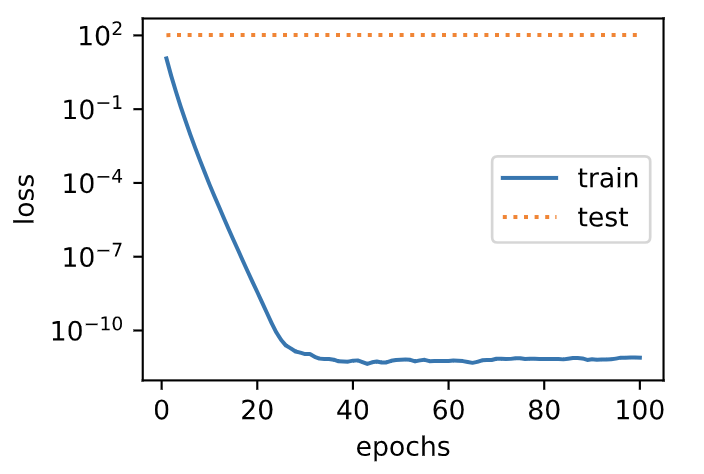
Next, let's train and test the high-dimensional linear regression model. When lambd is set to 0, we do not use weight attenuation. Results the training error is much smaller than the error on the test set.

This is a typical over fitting phenomenon.

fit_and_plot(lambd=0)

Output:

L2 norm of w: 15.114808082580566

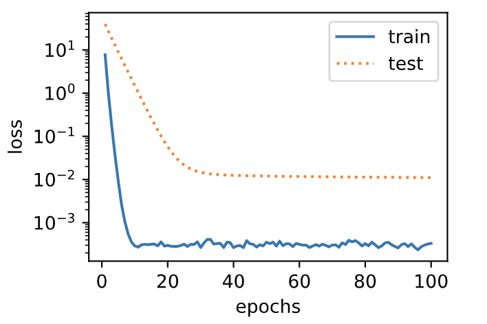
Use weight falloff

Let's use weight attenuation. It can be seen that although the training error is improved, the error on the test set is reduced. The over fitting phenomenon has been alleviated to a certain extent.

In addition, the weight parameter L 2 L_2 L2} norm is smaller than that without weight attenuation, and the weight parameter is closer to 0.

fit_and_plot(lambd=3)

Output:

L2 norm of w: 0.035220853984355927

Concise implementation

Here, we directly use weight when constructing the optimizer instance_ The decay parameter to specify the weight attenuation super parameter.

By default, PyTorch attenuates both weights and deviations. We can construct optimizer instances for weights and deviations respectively, so that only weights are attenuated.

def fit_and_plot_pytorch(wd):
    # Falloff the weight parameter. Weight names usually end with weight
    net = nn.Linear(num_inputs, 1)
    nn.init.normal_(net.weight, mean=0, std=1)
    nn.init.normal_(net.bias, mean=0, std=1)
    optimizer_w = torch.optim.SGD(params=[net.weight], lr=lr, weight_decay=wd) # Attenuation of weight parameters
    optimizer_b = torch.optim.SGD(params=[net.bias], lr=lr)  # No attenuation of deviation parameters
    
    train_ls, test_ls = [], []
    for _ in range(num_epochs):
        for X, y in train_iter:
            l = loss(net(X), y).mean()
            optimizer_w.zero_grad()
            optimizer_b.zero_grad()
            
            l.backward()
            
            # Call the step function on the two optimizer instances to update the weight and deviation respectively
            optimizer_w.step()
            optimizer_b.step()
        train_ls.append(loss(net(train_features), train_labels).mean().item())
        test_ls.append(loss(net(test_features), test_labels).mean().item())
    d2l.semilogy(range(1, num_epochs + 1), train_ls, 'epochs', 'loss',
                 range(1, num_epochs + 1), test_ls, ['train', 'test'])
    print('L2 norm of w:', net.weight.data.norm().item())

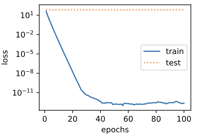
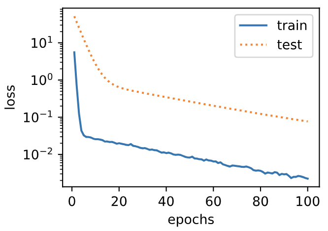
Similar to the experimental phenomenon of weight attenuation from zero, using weight attenuation can alleviate the over fitting problem to a certain extent.

fit_and_plot_pytorch(0)

Output:

L2 norm of w: 12.86785888671875

fit_and_plot_pytorch(3)

Output:

L2 norm of w: 0.09631537646055222

Summary

• Regularization makes the learned model parameters smaller by adding penalty terms to the model loss function, which is a common means to deal with over fitting.
• Weight attenuation is equivalent to L 2 L_2 L2} norm regularization usually makes the learned elements of weight parameters close to 0.
• Weight attenuation can be achieved by weight in the optimizer_ The decaly super parameter.
• Multiple optimizer instances can be defined to use different iterative methods for different model parameters.

Note: this section is basically the same as the original book except for the code, Original book portal

For the purpose of learning, I quote the content of this book for non-commercial purposes. I recommend you to read this book and study together!!!

come on.

thank!

strive!