Regression analysis -- multiple regression

Introduce the statistics in multiple regression analysis

• Total observed value
• Total independent variable
• Freedom: return degrees of freedom, residual degrees of freedom
• Sum of total square of SST
• Sum of squares of SSR regression
• Sum of squares of SSE residuals
• MSR mean square regression
• MSE mean square residual
• Determination coefficient R ﹣ square
• Adjusted? R? Square
• Multiple? R
• Standard error of estimation
• F-test statistics
• Standard error of sampling distribution of regression coefficient
• t-test statistics of regression coefficients
• Confidence interval of each regression coefficient
• log likelihood

• AIC guidelines
• BIC guidelines

Case analysis and python practice

# Import related packages
import pandas as pd
import numpy as np
import math
import scipy
import matplotlib.pyplot as plt
from scipy.stats import t

# Building data
columns = {'A':"Branch number", 'B':"Non-performing Loan(Billion yuan)", 'C':"Loan balance(Billion yuan)", 'D':"Accumulated loans receivable(Billion yuan)", 'E':"Number of loan items", 'F':"Fixed assets investment(Billion yuan)"}
data={"A":[1,2,3,4,5,6,7,8,9,10,11,12,13,14,15,16,17,18,19,20,21,22,23,24,25],
      "B":[0.9,1.1,4.8,3.2,7.8,2.7,1.6,12.5,1.0,2.6,0.3,4.0,0.8,3.5,10.2,3.0,0.2,0.4,1.0,6.8,11.6,1.6,1.2,7.2,3.2],
      "C":[67.3,111.3,173.0,80.8,199.7,16.2,107.4,185.4,96.1,72.8,64.2,132.2,58.6,174.6,263.5,79.3,14.8,73.5,24.7,139.4,368.2,95.7,109.6,196.2,102.2],
      "D":[6.8,19.8,7.7,7.2,16.5,2.2,10.7,27.1,1.7,9.1,2.1,11.2,6.0,12.7,15.6,8.9,0,5.9,5.0,7.2,16.8,3.8,10.3,15.8,12.0],
      "E":[5,16,17,10,19,1,17,18,10,14,11,23,14,26,34,15,2,11,4,28,32,10,14,16,10],
      "F":[51.9,90.9,73.7,14.5,63.2,2.2,20.2,43.8,55.9,64.3,42.7,76.7,22.8,117.1,146.7,29.9,42.1,25.3,13.4,64.3,163.9,44.5,67.9,39.7,97.1]
     }

df = pd.DataFrame(data)
X = df[["C", "D", "E", "F"]]
Y = df[["B"]]

# Building multiple linear regression model
from sklearn.linear_model import LinearRegression
lreg = LinearRegression()
lreg.fit(X, Y)

x = X
y_pred = lreg.predict(X)
y_true = np.array(Y).reshape(-1,1)

coef = lreg.coef_[0]
intercept = lreg.intercept_[0]

# Custom function
def log_like(y_true, y_pred):
    """
    y_true: True value
    y_pred: predicted value
    """
    sig = np.sqrt(sum((y_true - y_pred)**2)[0] / len(y_pred)) # Residual standard deviation δ
    y_sig = np.exp(-(y_true - y_pred) ** 2 / (2 * sig ** 2)) / (math.sqrt(2 * math.pi) * sig)
    loglik = sum(np.log(y_sig))
    return loglik

def param_var(x):
    """
    x:Only independent variable wide table
    """
    n = len(x)
    beta0 = np.ones((n,1))
    df_to_matrix = x.as_matrix()
    concat_matrix = np.hstack((beta0, df_to_matrix))         # Matrix merging
    transpose_matrix = np.transpose(concat_matrix)           # Matrix transposition
    dot_matrix = np.dot(transpose_matrix, concat_matrix)     # (X.T X)^(-1)
    inv_matrix = np.linalg.inv(dot_matrix)                   # Find (X.T X)^(-1) inverse matrix
    diag = np.diag(inv_matrix)                               # Obtain the diagonal of the matrix, i.e. the variance of each parameter
    return diag

def param_test_stat(x, Se, intercept, coef, alpha=0.05):
    n = len(x)
    k = len(x.columns)
    beta_array = param_var(x)
    beta_k = beta_array.shape[0]
    
    coef = [intercept] + list(coef)
    std_err = []
    t_Stat = []
    P_value = []
    t_intv = []
    coefLower = []
    coefupper = []
    
    for i in range(beta_k):
        se_belta = np.sqrt(Se**2 * beta_array[i])            # Sampling standard error of regression coefficient
        t = coef[i] / se_belta                               # T statistic used to test regression coefficient, i.e. test statistic t
        p_value = scipy.stats.t.sf(np.abs(t), n-k-1)*2       # P value used to test regression coefficient
        t_score = scipy.stats.t.isf(alpha/2, df = n-k-1)     # t critical value
        coef_lower = coef[i] - t_score * se_belta            # Lower confidence interval limit of regression coefficient (slope)
        coef_upper = coef[i] + t_score * se_belta            # Upper limit of confidence interval of regression coefficient (slope)
        
        std_err.append(round(se_belta, 3))
        t_Stat.append(round(t,3))
        P_value.append(round(p_value,3))
        t_intv.append(round(t_score,3))
        coefLower.append(round(coef_lower,3))
        coefupper.append(round(coef_upper,3))
        
    dict_ = {"coefficients":list(map(lambda x:round(x, 4), coef)), 
             'std_err':std_err, 
             't_Stat':t_Stat, 
             'P_value':P_value, 
             't critical value':t_intv, 
             'Lower_95%':coefLower, 
             'Upper_95%':coefupper}
    
    index = ["intercept"] + list(x.columns)
    stat = pd.DataFrame(dict_, index=index)
    return stat

# Custom function (calculate and output statistics of regression analysis)
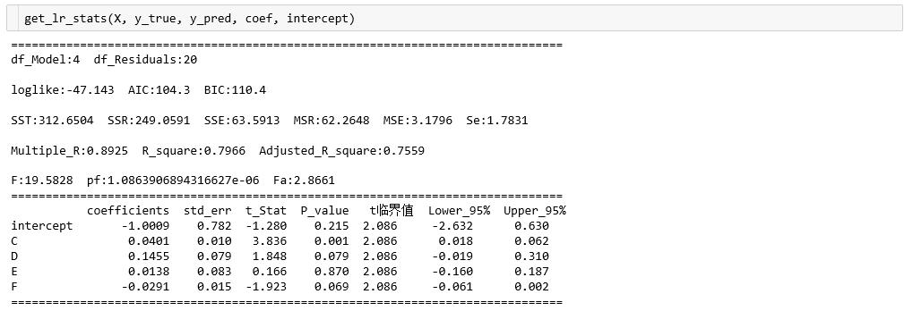
def get_lr_stats(x, y_true, y_pred, coef, intercept, alpha=0.05):
    
    n   = len(x)
    k   = len(x.columns)
    ssr = sum((y_pred - np.mean(y_true))**2)[0]  # Regression square sum SSR
    sse = sum((y_true - y_pred)**2)[0]           # Sum of squared residuals SSE
    sst = ssr + sse                              # Total square sum SST
    msr = ssr / k                                # Mean square regression MSR
    mse = sse / (n-k-1)                          # Mean square residual MSE
    
    R_square = ssr / sst                                   # Determination coefficient R^2
    Adjusted_R_square = 1-(1-R_square)*((n-1) / (n-k-1))   # Determination coefficient of adjustment
    Multiple_R = np.sqrt(R_square)                         # Complex correlation coefficient   
    Se = np.sqrt(sse/(n - k - 1))                          # Standard error of estimation
    
    loglike = log_like(y_true, y_pred)[0]
    AIC = 2*(k+1) - 2 * loglike                  # (k+1) represents k regression parameters or coefficients and 1 intercept parameter
    BIC = -2*loglike + (k+1)*np.log(n)  
    
    # Significance test of linear relationship
    F  = (ssr / k) / (sse / ( n - k - 1 ))            # Test statistic F (test of linear relationship)
    pf = scipy.stats.f.sf(F, k, n-k-1)                # Significance F for test, i.e. significance F
    Fa = scipy.stats.f.isf(alpha, dfn=k, dfd=n-k-1)   # F critical value
    
    # Significance test of regression coefficient
    stat = param_test_stat(x, Se, intercept, coef, alpha=alpha)
    
    # Output statistics of regression analysis
    print('='*80)
    print('df_Model:{}  df_Residuals:{}'.format(k, n-k-1), '\n')
    print('loglike:{}  AIC:{}  BIC:{}'.format(round(loglike,3), round(AIC,1), round(BIC,1)), '\n')
    print('SST:{}  SSR:{}  SSE:{}  MSR:{}  MSE:{}  Se:{}'.format(round(sst,4),
                                                                 round(ssr,4),
                                                                 round(sse,4),
                                                                 round(msr,4),
                                                                 round(mse,4),
                                                                 round(Se,4)), '\n')
    
    print('Multiple_R:{}  R_square:{}  Adjusted_R_square:{}'.format(round(Multiple_R,4),
                                                                    round(R_square,4),
                                                                    round(Adjusted_R_square,4)), '\n')
    print('F:{}  pf:{}  Fa:{}'.format(round(F,4), pf, round(Fa,4)))
    
    print('='*80)
    print(stat)
    print('='*80)
    
    return 0

The output results are as follows:

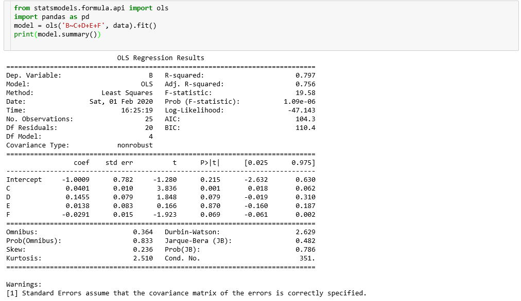
Compared with ols results under statsmodels: