Title Requirements

1. Complete the following requirements as required.
Use python to write the following program,
To gain a better understanding of univariate linear regression, we now design our own datasets.The requirements of the dataset are as follows: XDATA is 200 random numbers in the (0,5) range that obey the normal distribution, ydata satisfies: ydata=4*xdata+8+random1, where random1 is also a random number in the (0,5) range that obeys the normal distribution.Test Set: Select the first 50 data from the training set as the test set.Implement a linear regression model in Python and use it to predict y with the following requirements:
1. Generate training set data (8 points)
2. Generate test set data (8 points)
3. Cost function for linear regression (8 points)
4. Implement the gradient descent function (4 points)
5. Calculate the regression model by gradient descent, and use the model to predict (4 points) the data of the test set.
6. Draw scatter plots to compare the true values along the horizontal axis with the predicted values along the vertical axis (8 points)

Topic resolution

This topic requires us to generate our own data, so think clearly.Univariate linear regression is a handwritten bottom level, which is easy to examine, but can not be inadvertent. The important point is the adjustment of learning rate.

The implementation code is as follows:

'''
    //Handwritten Linear Regression
'''
import numpy as np
from matplotlib import pyplot as plt
# Set up normal display of Chinese fonts and minus sign
plt.rcParams['font.sans-serif'] = ['SimHei']
plt.rcParams['axes.unicode_minus'] = False
# design data
X = [np.random.normal(0,5) for _ in range(500)]
y = []
for i in X:
    y.append(4 * i + 8 + np.random.normal(0,5))

# 1. Generate training set data (8 points)
# Initialize data
m = len(X)
X = np.c_[np.ones(m),X]
y = np.c_[y]

# Select the first 50 data from the training set as the test set.# 2. Generate test set data (8 points)
X_test = X[0:50,:]
y_test = y[0:50,:]


# Define Model
def model(X,theta):
    h = np.dot(X,theta)
    return h


# Define cost function
def cost_function(h,y):
    m = len(h)
    J = 1/(2 * m) * np.sum(np.square(h - y))
    return J


# Define gradient descent
def gradeDesc(X,y,alpha=0.001,iter_max=10000):
    # Data preparation
    m,n = X.shape
    # Initialization
    J_history = np.zeros(iter_max)
    theta = np.zeros((n,1))
    # Perform Gradient Decrease
    for i in range(iter_max):
        h = model(X,theta)
        J_history[i] = cost_function(h,y)
        deltaTheta = 1/m * np.dot(X.T,h-y)
        theta -= alpha * deltaTheta
    return J_history,theta


# Calling the gradient descent function
J_history,theta = gradeDesc(X,y)
# 5. Calculate the regression model by gradient descent, and use the model to predict (4 points) the data of the test set.
y_test_h = model(X_test,theta)


# Define Accuracy Function
def score(h,y):
    u = np.sum(np.square(h - y))
    v = np.sum(np.square(y - np.mean(y)))
    return 1 - u/v


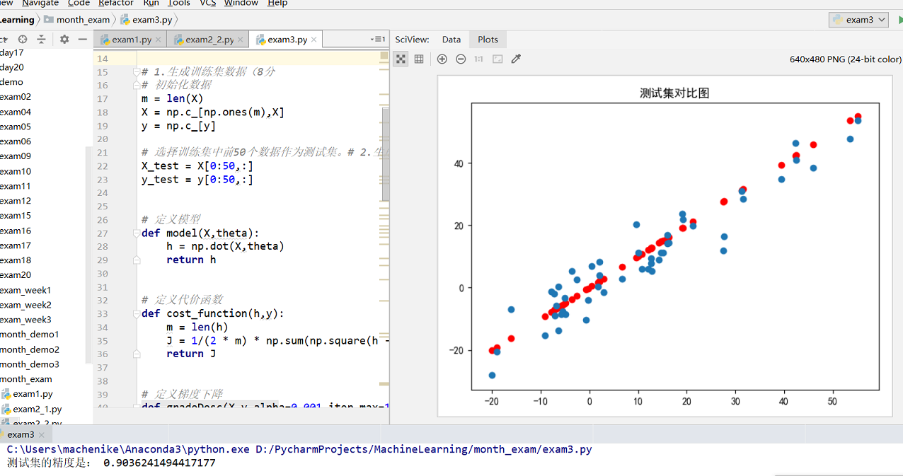
print('The precision of the test set is:',score(y_test_h,y_test))


# Draw cost function curve
plt.title('Cost function curve')
plt.plot(J_history)
plt.show()
# 6. Draw scatter plots to compare the true values along the horizontal axis with the predicted values along the vertical axis (8 points)
plt.title('Test Set Diagram')
plt.scatter(y_test,y_test,c='r')
plt.scatter(y_test,y_test_h)
plt.show()

The results are as follows: