Monte Carlo simulation for European option pricing

   for the European call option whose underlying asset price is S0 and execution price is X, the price of maturity t is CT = max(0,ST-X). In the risk neutral world, the option price at time t is CT = e-r(T-t)E[max(0,ST-X)], which is also one of the derivation ideas of BS formula. Because CT is only related to ST, we only need to simulate the path of ST, repeat n times, and then average them to get the price of call option, that is, CT = e-r(T-t) ∑ [max(0,ST-X)] /n, similarly, the price of put option PT = e-r(T-t) ∑ [max(0,X-ST)] /n. Note that Monte Carlo simulation cannot price American options.

Monte Carlo simulation of the subject asset price ST (23) It has been introduced in, mainly using the following formula: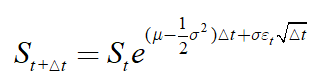

   suppose there is a stock option with a term of six months, the stock price of the underlying asset is 5.29 yuan, the execution price of the option is 6 yuan, the annualized risk-free interest rate and annualized volatility are 4% and 24% respectively, and the price of call option and put option is calculated by Monte Carlo simulation method (10000 times of simulation).

import numpy as np
from numpy.random import standard_normal
def callMonteCarlo(S,X,r,sigma,t,n):
	z=standard_normal(n)
	St=S*np.exp((r-0.5*sigma**2)*t+sigma*z*np.sqrt(t))
	return sum(np.maximum(0,St-X))*(np.exp(-r*t))/n
def putMonteCarlo(S,X,r,sigma,t,n):
	z=standard_normal(n)
	St=S*np.exp((r-0.5*sigma**2)*t+sigma*z*np.sqrt(t))
	return sum(np.maximum(0,X-St))*(np.exp(-r*t))/n
c=callMonteCarlo(5.29,6,0.04,0.24,0.5,10000)
p=putMonteCarlo(5.29,6,0.04,0.24,0.5,10000)
print('The call option price calculated by Monte Carlo simulation is{:.4f},Put option price is{:.4f}'.format(c,p))

//The call option price calculated by Monte Carlo simulation is0.1520,Put option price is0.7450

The price of call option and put option calculated by BS formula is 0.1532 and 0.7443 respectively. The result is very close.

The accuracy of   Monte Carlo simulation is proportional to the simulation times, but the increase of the times will reduce the calculation efficiency, so the stability can be improved and the simulation times can be reduced by the variance reduction technology. The main variance reduction techniques include dual variable technique and control variable technique.

Dual variable Monte Carlo simulation

The idea of    dual variable method is to generate N random numbers into the formula to obtain the average price of n samples, then make the other N random numbers as the opposite number of this group of random numbers to calculate the average price of n samples, and finally average the two prices. Because if one group of z is too large, the price calculated by the other group of z will be too small, and the average value of the two will be closer to the real situation. Take the above example:

def call_dual(S,X,r,sigma,t,n):
	z=standard_normal(n)
	S1=S*np.exp((r-0.5*sigma**2)*t+sigma*z*np.sqrt(t))
	S2=S*np.exp((r-0.5*sigma**2)*t+sigma*(-z)*np.sqrt(t))
	c1=sum(np.maximum(0,S1-X))*(np.exp(-r*t))/n
	c2=sum(np.maximum(0,S2-X))*(np.exp(-r*t))/n
	return (c1+c2)/2
def put_dual(S,X,r,sigma,t,n):
	z=standard_normal(n)
	S1=S*np.exp((r-0.5*sigma**2)*t+sigma*z*np.sqrt(t))
	S2=S*np.exp((r-0.5*sigma**2)*t+sigma*(-z)*np.sqrt(t))
	c1=sum(np.maximum(0,X-S1))*(np.exp(-r*t))/n
	c2=sum(np.maximum(0,X-S2))*(np.exp(-r*t))/n
	return (c1+c2)/2
c=call_dual(5.29,6,0.04,0.24,0.5,5000)
p=put_dual(5.29,6,0.04,0.24,0.5,5000)
print('The price of call option calculated by dual Monte Carlo method is{:.4f},Put option price is{:.4f}'.format(c,p))

//The price of call option calculated by dual Monte Carlo method is0.1526,Put option price is0.7438

It can be seen that under the dual Monte Carlo simulation method, the result of only 5000 simulations is very close to that of BS formula.

Monte Carlo simulation of control variables

   if the price of derivative a is highly correlated with that of derivative B, and the price of B is known or easy to estimate, then after estimating B by Monte Carlo method, the error can be added to the Monte Carlo estimate of A. The disadvantage of this method is to find B which has a high correlation with a. The specific code can be designed as follows (in which the price of option B is parameter B and the price of the underlying asset is S2):

def call_con(S1,S2,X,r,sigma,t,B,n):
	z1=standard_normal(n)
	S1t=S1*np.exp((r-0.5*sigma**2)*t+sigma*z*np.sqrt(t))
	C1=sum(np.maximum(0,S1t-X))*(np.exp(-r*t))/n
	z2=standard_normal(n)
	S2t=S2*np.exp((r-0.5*sigma**2)*t+sigma*z*np.sqrt(t))
	C2=sum(np.maximum(0,S2t-X))*(np.exp(-r*t))/n
	return C1+B-C2

In conclusion, I think dual Monte Carlo simulation is the most cost-effective method.