In previous Demo, we used conditional GAN to generate handwritten digital images.So what else can we do with neural networks in addition to generating digital images?
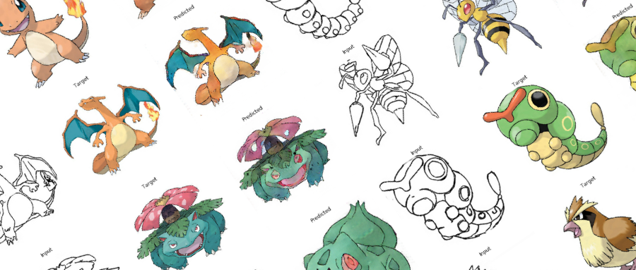
In this case, we use a neural network to color the wireframe of the Pocket Monster.
Step 1: Import Usage Library
from __future__ import absolute_import, division, print_function, unicode_literals

import tensorflow as tf
tf.enable_eager_execution()

import numpy as np
import pandas as pd

import os
import time
import matplotlib.pyplot as plt
from IPython.display import clear_output
A larger memory is required during the model training for Pocket Monster coloring.To ensure that our model runs smoothly on 2070, we limit the usage of video memory to 90% to avoid errors caused by insufficient video memory.
config = tf.compat.v1.ConfigProto()
config.gpu_options.per_process_gpu_memory_fraction = 0.9
session = tf.compat.v1.Session(config=config)
Define the constants you need to use.
BUFFER_SIZE = 400
BATCH_SIZE = 1
IMG_WIDTH = 256
IMG_HEIGHT = 256
PATH = 'dataset/'
OUTPUT_CHANNELS = 3
LAMBDA = 100
EPOCHS = 10
Step 2: Define the function you want to use
Picture data loading function, the main purpose is to use the io interface of Tensorflow to read pictures and put them into tensor's object for subsequent use
def load(image_file):
    image = tf.io.read_file(image_file)
    image = tf.image.decode_jpeg(image)

    w = tf.shape(image)[1]

    w = w // 2
    input_image = image[:, :w, :]
    real_image = image[:, w:, :]

    input_image = tf.cast(input_image, tf.float32)
    real_image = tf.cast(real_image, tf.float32)

    return input_image, real_image
Functions that convert tensor objects to numpy objects
During the training, I will visualize some training results and pictures of the intermediate state.Tensorflow's tensor object cannot be used directly in matplot, so we need a function to convert tensor to a numpy object.
def tensor_to_array(tensor1):
    return tensor1.numpy()
Step 3: Data visualization
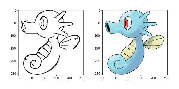
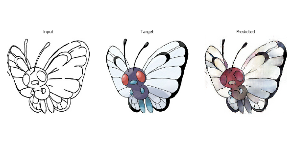
Let's first see how our training data looks. Each data picture is divided into two parts, the left part is a wireframe, we use it as input data, the right part is a color map, and we use it as training target picture. Let's use the load function defined above to load a picture and see
input, real = load(PATH+'train/114.jpg')

plt.figure()
plt.imshow(tensor_to_array(input)/255.0)
plt.figure()
plt.imshow(tensor_to_array(real)/255.0)
Step 4: Data Enhancement
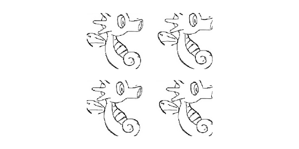
Because we don't have enough training data, we use data enhancement to increase our sample size.Thus, small sample data can also achieve better results.
We take the following data enhancement schemes:
- Picture zoom, zoom the picture of the input data to the size of the picture we specified
- Random clipping
- data normalization
- Flip
def resize(input_image, real_image, height, width):
    input_image = tf.image.resize(input_image, [height, width], method=tf.image.ResizeMethod.NEAREST_NEIGHBOR)
    real_image = tf.image.resize(real_image, [height, width], method=tf.image.ResizeMethod.NEAREST_NEIGHBOR)

    return input_image, real_image
def random_crop(input_image, real_image):
    stacked_image = tf.stack([input_image, real_image], axis=0)
    cropped_image = tf.image.random_crop(stacked_image, size=[2, IMG_HEIGHT, IMG_WIDTH, 3])

    return cropped_image[0], cropped_image[1]
def random_crop(input_image, real_image):
    stacked_image = tf.stack([input_image, real_image], axis=0)
    cropped_image = tf.image.random_crop(stacked_image, size=[2, IMG_HEIGHT, IMG_WIDTH, 3])

    return cropped_image[0], cropped_image[1]
We form a function of the above enhancement scheme, where left-right flipping occurs randomly
@tf.function()
def random_jitter(input_image, real_image):
    input_image, real_image = resize(input_image, real_image, 286, 286)
    input_image, real_image = random_crop(input_image, real_image)

    if tf.random.uniform(()) > 0.5:
        input_image = tf.image.flip_left_right(input_image)
        real_image = tf.image.flip_left_right(real_image)

    return input_image, real_image
Effect of data enhancement
plt.figure(figsize=(6, 6))
for i in range(4):
    input_image, real_image = random_jitter(input, real)
    plt.subplot(2, 2, i+1)
    plt.imshow(tensor_to_array(input_image)/255.0)
    plt.axis('off')
plt.show()
Step 5: Preparing training data
Define load functions for training and test data
def load_image_train(image_file):
    input_image, real_image = load(image_file)
    input_image, real_image = random_jitter(input_image, real_image)
    input_image, real_image = normalize(input_image, real_image)

    return input_image, real_image
def load_image_test(image_file):
    input_image, real_image = load(image_file)
    input_image, real_image = resize(input_image, real_image, IMG_HEIGHT, IMG_WIDTH)
    input_image, real_image = normalize(input_image, real_image)

    return input_image, real_image
Use tensorflow's DataSet to load training and test data, define our training data and test dataset objects
train_dataset = tf.data.Dataset.list_files(PATH+'train/*.jpg')
train_dataset = train_dataset.map(load_image_train, num_parallel_calls=tf.data.experimental.AUTOTUNE)
train_dataset = train_dataset.cache().shuffle(BUFFER_SIZE)
train_dataset = train_dataset.batch(1)
test_dataset = tf.data.Dataset.list_files(PATH+'test/*.jpg')
test_dataset = test_dataset.map(load_image_test)
test_dataset = test_dataset.batch(1)
Step 6: Define the model
Pocket monster coloring, we used the GAN model to train, this time the GAN model is more complex to read than the previous conditional GAN produces handwritten digital pictures. Let's first look at the overall structure of the resulting and discriminant networks
Generate Network
Generating a network uses the basic framework of U-Net, the way we use Convolution Layer->BN Layer->LeakyReLU for each block in the coding phase.For each block in the decoding phase, we use Deconvolution->BN Layer->Dropout or ReLU.The first three blocks use Dropout, and the latter use ReLU.Block output from each encoding layer is also connected to the corresponding decoding layer's block. Refer specifically to skip connection from U-Net.
Define Coding Block
def downsample(filters, size, apply_batchnorm=True):
    initializer = tf.random_normal_initializer(0., 0.02)

    result = tf.keras.Sequential()
    result.add(tf.keras.layers.Conv2D(filters, size, strides=2, padding='same', kernel_initializer=initializer, use_bias=False))

    if apply_batchnorm:
        result.add(tf.keras.layers.BatchNormalization())

    result.add(tf.keras.layers.LeakyReLU())

    return result

down_model = downsample(3, 4)
Define Decode Block
def upsample(filters, size, apply_dropout=False):
    initializer = tf.random_normal_initializer(0., 0.02)

    result = tf.keras.Sequential()
    result.add(tf.keras.layers.Conv2DTranspose(filters, size, strides=2, padding='same', kernel_initializer=initializer, use_bias=False))
    result.add(tf.keras.layers.BatchNormalization())

    if apply_dropout:
        result.add(tf.keras.layers.Dropout(0.5))

    result.add(tf.keras.layers.ReLU())

    return result

up_model = upsample(3, 4)
Define Generate Network Model
def Generator():
    down_stack = [
        downsample(64, 4, apply_batchnorm=False), # (bs, 128, 128, 64)
        downsample(128, 4), # (bs, 64, 64, 128)
        downsample(256, 4), # (bs, 32, 32, 256)
        downsample(512, 4), # (bs, 16, 16, 512)
        downsample(512, 4), # (bs, 8, 8, 512)
        downsample(512, 4), # (bs, 4, 4, 512)
        downsample(512, 4), # (bs, 2, 2, 512)
        downsample(512, 4), # (bs, 1, 1, 512)
    ]

    up_stack = [
        upsample(512, 4, apply_dropout=True), # (bs, 2, 2, 1024)
        upsample(512, 4, apply_dropout=True), # (bs, 4, 4, 1024)
        upsample(512, 4, apply_dropout=True), # (bs, 8, 8, 1024)
        upsample(512, 4), # (bs, 16, 16, 1024)
        upsample(256, 4), # (bs, 32, 32, 512)
        upsample(128, 4), # (bs, 64, 64, 256)
        upsample(64, 4), # (bs, 128, 128, 128)
    ]

    initializer = tf.random_normal_initializer(0., 0.02)
    last = tf.keras.layers.Conv2DTranspose(OUTPUT_CHANNELS, 4,
                                         strides=2,
                                         padding='same',
                                         kernel_initializer=initializer,
                                         activation='tanh') # (bs, 256, 256, 3)

    concat = tf.keras.layers.Concatenate()

    inputs = tf.keras.layers.Input(shape=[None,None,3])
    x = inputs

    skips = []
    for down in down_stack:
        x = down(x)
        skips.append(x)

    skips = reversed(skips[:-1])

    for up, skip in zip(up_stack, skips):
        x = up(x)
        x = concat([x, skip])

    x = last(x)

    return tf.keras.Model(inputs=inputs, outputs=x)

generator = Generator()
Discriminant Network
Discriminant networks we use PatchGAN, also known as Markov discriminator.Many of the traditional CNN-based classification models introduce a fully connected layer at the end, and then output the results of the discrimination.However, PatchGAN is not the same. It consists entirely of convolution layers, and the final output is a square array with a latitude of N.Then the mean of the matrix is calculated as true or false output.Visually, each output of the output square matrix is a field of the model's perception in the original map, which corresponds to a place in the original map, also known as Patch. Therefore, the GAN of this structure is called PatchGAN.
Each Block in PatchGAN is made up of convolution layer->BN layer->Leaky ReLU.
In our model, the last level of latitude of our output is (Batch Size, 30, 30, 1), where 1 represents the channel of the picture.
Each 30x30 output corresponds to the 70x70 area of the original map.Detailed structure can be referenced in this article paper.
def Discriminator():
    initializer = tf.random_normal_initializer(0., 0.02)

    inp = tf.keras.layers.Input(shape=[None, None, 3], name='input_image')
    tar = tf.keras.layers.Input(shape=[None, None, 3], name='target_image')

    # (batch size, 256, 256, channels*2)
    x = tf.keras.layers.concatenate([inp, tar])

    # (batch size, 128, 128, 64)
    down1 = downsample(64, 4, False)(x)

    # (batch size, 64, 64, 128)
    down2 = downsample(128, 4)(down1)

    # (batch size, 32, 32, 256)
    down3 = downsample(256, 4)(down2)

    # (batch size, 34, 34, 256)
    zero_pad1 = tf.keras.layers.ZeroPadding2D()(down3)

    # (batch size, 31, 31, 512)
    conv = tf.keras.layers.Conv2D(512, 4, strides=1, kernel_initializer=initializer, use_bias=False)(zero_pad1)

    batchnorm1 = tf.keras.layers.BatchNormalization()(conv)

    leaky_relu = tf.keras.layers.LeakyReLU()(batchnorm1)

    # (batch size, 33, 33, 512)
    zero_pad2 = tf.keras.layers.ZeroPadding2D()(leaky_relu)

    # (batch size, 30, 30, 1)
    last = tf.keras.layers.Conv2D(1, 4, strides=1, kernel_initializer=initializer)(zero_pad2)

    return tf.keras.Model(inputs=[inp, tar], outputs=last)

discriminator = Discriminator()
Step 7: Define the loss function and optimizer
** **
loss_object = tf.keras.losses.BinaryCrossentropy(from_logits=True)
**
def discriminator_loss(disc_real_output, disc_generated_output):
    real_loss = loss_object(tf.ones_like(disc_real_output), disc_real_output)
    generated_loss = loss_object(tf.zeros_like(disc_generated_output), disc_generated_output)

    total_disc_loss = real_loss + generated_loss

    return total_disc_loss
def generator_loss(disc_generated_output, gen_output, target):
    gan_loss = loss_object(tf.ones_like(disc_generated_output), disc_generated_output)
    l1_loss = tf.reduce_mean(tf.abs(target - gen_output))

    total_gen_loss = gan_loss + (LAMBDA * l1_loss)

    return total_gen_loss
generator_optimizer = tf.keras.optimizers.Adam(2e-4, beta_1=0.5)
discriminator_optimizer = tf.keras.optimizers.Adam(2e-4, beta_1=0.5)
Step 8: Define the CheckPoint function
Because our training takes a long time, we will save the middle training state for subsequent loading to continue training.
checkpoint = tf.train.Checkpoint(generator_optimizer=generator_optimizer,
                                 discriminator_optimizer=discriminator_optimizer,
                                 generator=generator,
                                 discriminator=discriminator)
If we save the results of previous training, we load the saved data.Then we apply the last saved model to output our test data.
def generate_images(model, test_input, tar):
    prediction = model(test_input, training=True)
    plt.figure(figsize=(15,15))

    display_list = [test_input[0], tar[0], prediction[0]]
    title = ['Input', 'Target', 'Predicted']

    for i in range(3):
        plt.subplot(1, 3, i+1)
        plt.title(title[i])
        plt.imshow(tensor_to_array(display_list[i]) * 0.5 + 0.5)
        plt.axis('off')
    plt.show()
ckpt_manager = tf.train.CheckpointManager(checkpoint, "./", max_to_keep=2)

if ckpt_manager.latest_checkpoint:
    checkpoint.restore(ckpt_manager.latest_checkpoint)

for inp, tar in test_dataset.take(20):
    generate_images(generator, inp, tar)
Step 9: Training
During the training, we output the first picture to see how each epoch changes our predictions.Let everyone enjoy it We save the status every 20 epoch s
@tf.function
def train_step(input_image, target):
    with tf.GradientTape() as gen_tape, tf.GradientTape() as disc_tape:
        gen_output = generator(input_image, training=True)

        disc_real_output = discriminator([input_image, target], training=True)
        disc_generated_output = discriminator([input_image, gen_output], training=True)

        gen_loss = generator_loss(disc_generated_output, gen_output, target)
        disc_loss = discriminator_loss(disc_real_output, disc_generated_output)

    generator_gradients = gen_tape.gradient(gen_loss,
                                          generator.trainable_variables)
    discriminator_gradients = disc_tape.gradient(disc_loss,
                                               discriminator.trainable_variables)

    generator_optimizer.apply_gradients(zip(generator_gradients,
                                          generator.trainable_variables))
    discriminator_optimizer.apply_gradients(zip(discriminator_gradients,
                                              discriminator.trainable_variables))
def fit(train_ds, epochs, test_ds):
    for epoch in range(epochs):
        start = time.time()

        for input_image, target in train_ds:
            train_step(input_image, target)

        clear_output(wait=True)

        for example_input, example_target in test_ds.take(1):
            generate_images(generator, example_input, example_target)

        if (epoch + 1) % 20 == 0:
            ckpt_save_path = ckpt_manager.save()
            print ('Save{}individual epoch reach{}\n'.format(epoch+1, ckpt_save_path))

        print ('Training session{}individual epoch The time taken is{:.2f}second\n'.format(epoch + 1, time.time()-start))
fit(train_dataset, EPOCHS, test_dataset)
The time taken to train the eighth epoch was 51.33 seconds.
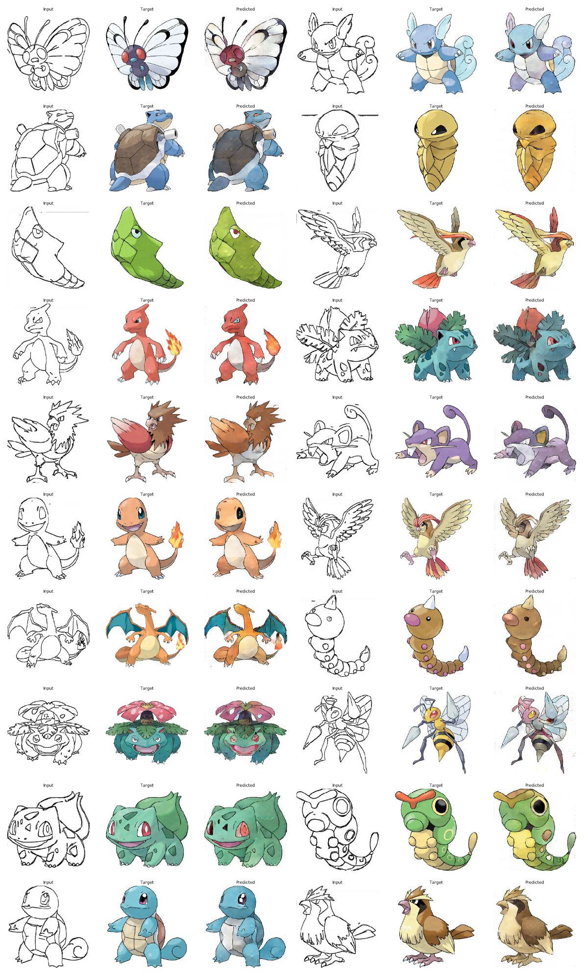
Step 10: Coloring the test data to see our results
for input, target in test_dataset.take(20):
    generate_images(generator, input, target)
Moment pool cloud Now on the shelf is a "Pocket Monster Colored" mirror; Moment Pool Cloud is dedicated to building the world's leading open artificial intelligence computing platform.Small partners of interest can try it out in the Jupyter Tutorial Demo mirror on Moment Pool Cloud's official website.