Still follow @Sichuan rookie Punch in · the next day
Article catalog
1. Use the knowledge learned on the first day to solve:
2. Understanding of this question:
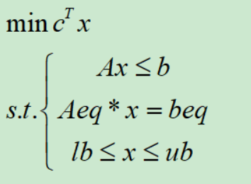
Basic theory (problem solving steps):
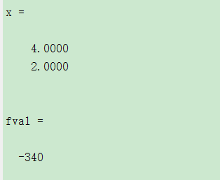
Result 1: optimal solution: x1 = 4, x2 = 2; Optimal value: 340
Result 2: optimal solution: x1 = 4, x2 = 2; Optimal value: 340
1, This question
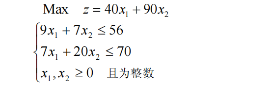
1. Use the knowledge learned on the first day to solve:
Modeling learning punch in day one_ Caicai stupid child's blog - CSDN blog

The code is as follows:
%Punch in the first day
clear all
clc
c=[40 90];%Determined by objective function coefficient
a=[9 7 ;7 20];%Inequality constraint
b=[56 70];%Right coefficient of inequality constraint
aeq=[];%There are no equality constraints, so aeq,beq All empty
beq=[];
lb=[0;0];%No lower limit
ub=[inf;inf];%No upper limit
[x,fval]=linprog(-c,a,b,aeq,beq,lb,ub);
x  %Get corresponding x1,x2
best=c*x%Calculate the optimal value
2. Understanding of this question:
Since the problem requires the solution results to be integers, the first question has the wrong result, so how can we get the desired integer solution?
(1) Branch definition method
Background:
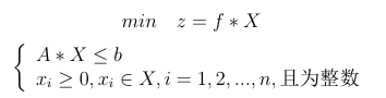
Today, matlab is used to realize the branch and bound method for solving complete integer programming problems. The model solved here is the objective function minimization model:
Basic theory (problem solving steps):
- Branch and bound method: a method for solving integer programming problems.
- Solution steps:
Firstly, we specify that the integer programming problem is A and the corresponding linear programming problem is B
- Solve problem B
1. If B has no feasible solution, A also has no feasible solution, stop the calculation
2. If B has an optimal solution and meets the integer condition, the optimal solution is the optimal solution of A, and the calculation is stopped
3. If B has an optimal solution but does not meet the integer condition, record its objective function value as z * as the lower bound of the optimal value - An integer feasible solution of problem A is found, and its objective function value is taken as the upper bound of the optimal solution
- Iterate
- Branch, select any variable x J X that does not meet the integer condition in the optimal solution of B_ JXJ, whose value is b j b_jbj, construct two constraints,
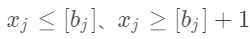 , respectively added to question B to form two sub questions B1 and B2. These two subproblems are solved without considering the integer condition. Branch
 - Delimit. The results of each subsequent problem are shown and compared with other problems. The minimum value of the optimal objective function (excluding problem B) is taken as the new lower bound. In each branch that meets the integer condition, the minimum value of the objective function is found as the new upper bound.
- Pruning: prune the branches whose objective function values are not in the upper and lower bounds
- Repeat 1, 2, 3 until the optimal solution is obtained
Note: when decomposing the two branches, give priority to the branch with the smallest objective function value for decomposition.
- Branch, select any variable x J X that does not meet the integer condition in the optimal solution of B_ JXJ, whose value is b j b_jbj, construct two constraints,
In the branch and bound method, the branches are pruned by delimitation, so that we can only seek the optimal solution in some feasible solutions, rather than exhaustive search, and its solution efficiency is higher.
Solution implementation 1:
See the meaning of linprog function and its parameters Modeling learning punch in day one_ Caicai stupid child's blog - CSDN blog
First of all, MATLAB solves the problem that the objective function is the minimum value, but if our objective function is to find the maximum value, we can convert the problem of finding the maximum value into the problem of finding the minimum value by multiplying each item of the objective function by - 1; A. b are the coefficient matrices in inequality constraints. Aeq and beq are coefficient matrices in equality constraints respectively, and lb and ub are upper and lower intervals of each variable respectively; Finally, c is the coefficient matrix of each variable in the objective function.
1. First, we need to define a function that satisfies the conditions of bifurcation theorem:
%A,b,c Corresponding to the inequality constraint coefficient matrix, inequality constraint constant vector and objective function coefficient vector respectively
%Aeq   Equality constraint coefficient matrix,   Beq    Equality constraint constant vector
%vlb   Define the lower bound of the domain        vub    Upper bound of definition field
%optXin   Optimal for each iteration x   optF   Optimal per iteration f value  iter Number of iterations

function [xstar, fxstar, flagOut, iter] = BranchBound1(c,A, b, Aeq, Beq, vlb, vub, optXin, optF, iter)
    global optX optVal optFlag;%The optimal solution is defined as a global variable
    iter = iter + 1;
    optX = optXin; optVal = optF;%Update the value from the iteration
    % options = optimoptions("linprog", 'Algorithm', 'interior-point-legacy', 'display', 'none');

    [x, fit, status] = linprog(c,A, b, Aeq, Beq, vlb, vub, []);
    %status Returns the reason why the algorithm iteration stopped
    %status = 1 The algorithm converges to the solution x,Namely x Is the optimal solution of linear programming
    if status ~= 1%If the optimal solution is not found, this branch does not need to continue to iterate and returns
        xstar = x;
        fxstar = fit;
        flagOut = status;
        return;
    end

    if max(abs(round(x) - x)) > 1e-3%The optimal solution of the function found is still not an integer solution
        if fit > optVal   %The solution to this problem is max,The function value at this time is greater than the value of the previous solution
            xstar = x;
            fxstar = fit;
            flagOut = -100;
            return;
        end

    else%At this time, the function solution obtained is an integer solution. The branch solution ends, and the downward solution is no longer continued. Return
        if fit > optVal   %The solution to this problem is max,The function value at this time is greater than the value of the previous solution
            xstar = x;
            fxstar = fit;
            flagOut = -101;
            return;
        else   %Solved value<The previously solved value is put into the global variable for temporary storage
            optVal = fit;
            optX = x;
            optFlag = status;
            xstar = x;
            fxstar = fit;
            flagOut = status;
            return;
        end
    end
    midX = abs(round(x) - x);%obtain x Corresponding decimal part
    notIntV = find(midX > 1e-3);%Get non integer x Index value of, find()The function returns an index value other than 0
    pXidx = notIntV(1);%Get the first non integer x Subscript index of
    tempVlb = vlb;%A temporary copy
    tempVub = vub;
    %fix(x) Function will x Zero direction rounding of elements in
    if vub(pXidx) >= fix(x(pXidx)) + 1%The original upper bound is greater than the position value of the boundary found at this time
        tempVlb(pXidx) = fix(x(pXidx)) + 1;%This boundary position value is passed in as a new lower bound parameter for further recursion
        [~, ~, ~] = BranchBound1(c,A, b, Aeq, Beq, tempVlb, vub, optX, optVal, iter + 1);
    end

    if vlb(pXidx) <= fix(x(pXidx))%The original lower bound is less than the position value of the boundary found at this time
        tempVub(pXidx) = fix(x(pXidx));%This boundary position value is passed in as a new upper bound parameter for further recursion
        [~, ~, ~] = BranchBound1(c,A, b, Aeq, Beq, vlb, tempVub, optX, optVal, iter + 1);
    end
    xstar = optX;
    fxstar = optVal;
    flagOut = optFlag;
end
2. Call the above function to solve the problem:
%A,b,c Corresponding to the inequality constraint coefficient matrix, inequality constraint constant vector and objective function coefficient vector respectively
%Aeq   Equality constraint coefficient matrix,   Beq    Equality constraint constant vector
%lb   Define the lower bound of the domain        ub    Upper bound of definition field

clear all
clc

A = [9 7;7 20];
b = [56 70];
c = [-40,-90];%The standard format is min,The title is max,It needs to be changed

lb = [0; 0];%x Lower bound of initial range of values
ub=[inf;inf];%x Upper bound of initial range of values

optX = [0; 0];%Storing the optimal solution x,Initial iteration point(0,0)
optVal = 0;%Optimal solution
[x, fit, exitF, iter] = BranchBound1(c,A, b,[], [], lb, ub, optX, optVal, 0)
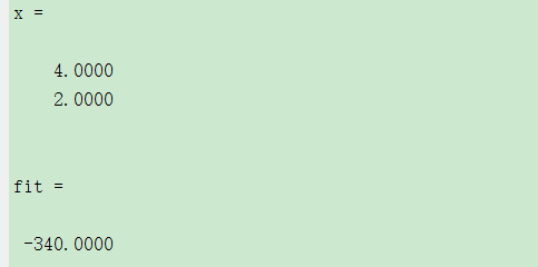
Result 1: optimal solution: x1 = 4, x2 = 2; Optimal value: 340
As for the negative result, it is because matlab solves the linear programming and turns it into finding the minimum value
Solution implementation 2:
See the meaning of linprog function and its parameters Modeling learning punch in day one_ Caicai stupid child's blog - CSDN blog
First of all, MATLAB solves the problem that the objective function is the minimum value, but if our objective function is to find the maximum value, we can convert the problem of finding the maximum value into the problem of finding the minimum value by multiplying each item of the objective function by - 1; A. b are the coefficient matrices in inequality constraints. Aeq and beq are coefficient matrices in equality constraints respectively, and lb and ub are upper and lower intervals of each variable respectively; Finally, c is the coefficient matrix of each variable in the objective function.
However, there are two special cases of linear norms, namely integer programming and 0-1 integer programming. Before (I don't know how long before Matlab...), matlab can't directly solve these two kinds of programming. bintprog function can be used to solve 0-1 integer programming, but the solving process is troublesome. Moreover, the latest version of MATLAB has abandoned this function and provided a relatively new function - intlinprog, which is dedicated to solving integer programming and 0-1 integer programming. A prototype of intlinprog is:
[x,fval,exitflag]= intlinprog(f,intcon,A,b,Aeq,beq,lb,ub)
The use of this function is very similar to the use of linprog function, which only adds one more parameter - intcon on the basis of linprog function. In the function intlinprog, intcon means the position of the integer constraint variable. In this question, the integer variables are x1 and x2, so intcon=[1,2]; fval is the optimized value, generally a scalar, and exitflag means the exit flag of the function.
The code of this question is as follows:
clear all
clc

c=[-40 -90];%Determined by objective function coefficient
A=[9 7;7 20];%Constraint left constraint
b=[56 70];%Constraint right coefficient
%lb=zeros(2,1);% Generate a full 0 matrix with 2 rows and 1 column,It's easy to see that in the above example x,y The minimum value of is 0
%intcon=[1,2];%Position of integer constraint variable
%[x,fval,exitflag]=intlinprog(c,intcon,A,b,[],[],lb,[]) %Use matrix lb No upper limit is required

lb=[0;0];%The lower limit is still 0
ub=[inf;inf];%x1 There is no upper limit, x2 No upper limit
intcon=[1,2];%Position of integer constraint variable
[x,fval,exitflag]=intlinprog(c,intcon,A,b,[],[],lb,ub) %At this time, the upper and lower limits need to be set
Result 2: optimal solution: x1 = 4, x2 = 2; Optimal value: 340
As for the negative result, it is because matlab solves the linear programming and turns it into finding the minimum value
Summary:
To sum up: optimal solution: x1 = 4, x2 = 2; Optimal value: 340 Is a positive solution; This time, I learned integer linear programming by learning the branch definition method. I learned it for a long time. Finally, my kung fu is worthy of my heart!! If there are errors in this article, please point out!! thank!