Model Tree and Project Case of 9.3 Tree Regression in Machine Learning Practice

All the codes in this article can be downloaded from github. You might as well have a Star to thank you. Github code address

I. Introduction

In this section, we introduce the model tree and a simple tree regression project.

2. Model Tree

Introduction of 2.1 Model Tree

The leaf node of regression tree is a constant value, while the leaf node of model tree is a regression equation.

In addition to simply setting leaf nodes as constant values, another way to model data with trees is to set leaf nodes as piecewise linear functions. In this case, piecewise linear means that the model consists of multiple linear segments.

Let's take a look at the data in the graph. Would it be better to model with two straight lines than with a set of constants? The answer is obvious. Two straight lines can be designed from 0.0-0.3 and 0.3-1.0 respectively, so two linear models can be obtained. Because part of the data set (0.0-0.3) is modeled by a linear model, while the other part (0.3-1.0) is modeled by another linear model, we use the so-called piecewise linear model.

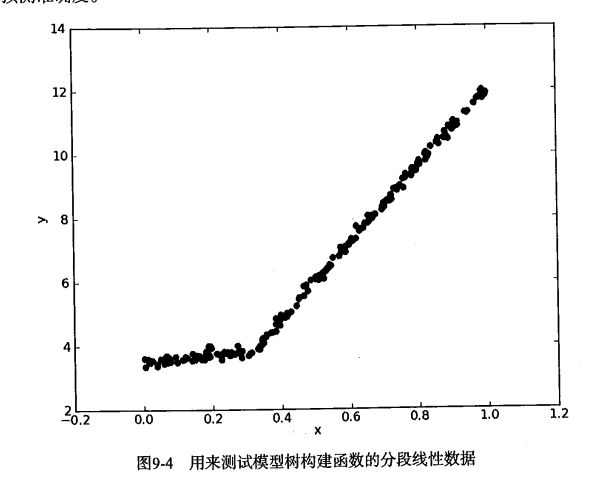
One of the advantages of decision tree over other machine learning algorithms is that the results are easier to understand. Obviously, two straight lines are easier to explain than many nodes forming a tree. Interpretability of model tree is one of the characteristics that it is superior to regression tree. In addition, the model tree also has higher prediction accuracy.

By slightly modifying the previous regression tree code, a linear model can be generated at leaf nodes instead of a constant value. Next, we will use the tree generation algorithm to partition the data, and each segmentation data can be easily represented by a linear model. The key of this algorithm lies in the calculation of error.

So in order to find the best segmentation, how should we calculate the error? The previous error calculation method for regression tree can not be used here. With a slight change, for a given data set, the model should be used to fit it first, and then the difference between the real target value and the model predicted value should be calculated. Finally, the required errors are obtained by summing the squares of these differences.

2.2. Model Tree Code

We created the modelTree.py file and wrote the following code

#!/usr/bin/env python
# -*- encoding: utf-8 -*-
'''
@File    :   modelTree.py
@Time    :   2019/08/12 14:47:06
@Author  :   xiao ming 
@Version :   1.0
@Contact :   xiaoming3526@gmail.com
@Desc    :   None
@github  :   https://github.com/aimi-cn/AILearners
'''

# here put the import lib
from numpy import *
import numpy as np
import matplotlib.pyplot as plt

'''
@description: Divide data sets according to features
@param: dataSet - Data aggregation
        feature - Characteristics with Segmentation
        value - The value of this feature
@return: mat0 - Segmented data set 0
        mat1 - Segmented data set 1
'''
def binSplitDataSet(dataSet, feature, value):
    mat0 = dataSet[np.nonzero(dataSet[:,feature] > value)[0],:]
    mat1 = dataSet[np.nonzero(dataSet[:,feature] <= value)[0],:]
    return mat0, mat1

'''
@description: Loading data
@param: fileName - file name 
@return: dataMat - Data Matrix
'''
def loadDataSet(fileName):
    dataMat = []
    fr = open(fileName)
    for line in fr.readlines():
        curLine = line.strip().split('\t')
        fltLine = list(map(float, curLine))                    #Convert to float type
        dataMat.append(fltLine)
    return dataMat

'''
@description: Draw ex00.txt data set
@paramL filename - file name
@return: None
'''
def plotDataSet(filename):
    dataMat = loadDataSet(filename)                                        #Loading data sets
    n = len(dataMat)                                                    #Number of data
    xcord = []; ycord = []                                                #Sample Points
    for i in range(n):                                                    
        xcord.append(dataMat[i][0]); ycord.append(dataMat[i][1])        #Sample Points
    fig = plt.figure()
    ax = fig.add_subplot(111)                                            #Add subplot
    ax.scatter(xcord, ycord, s = 20, c = 'blue',alpha = .5)                #Drawing sample points
    plt.title('DataSet')                                                #Draw title
    plt.xlabel('X')
    plt.show()

'''
@description: Generating leaf nodes
@param: dataSet - Data aggregation
@return: Means of target variables
'''
def regLeaf(dataSet):
    return np.mean(dataSet[:,-1])

'''
@description: Error Estimation Function
@param: dataSet - Data aggregation
@return: Total variance of target variables
'''
def regErr(dataSet):
    return np.var(dataSet[:,-1]) * np.shape(dataSet)[0]

'''
@description: Finding the Best Bivariate Segmentation Function for Data
@param:  dataSet - Data aggregation
        leafType - Generating leaf nodes
        regErr - Error Estimation Function
        ops - Tuples of user-defined parameters
@return:  bestIndex - Optimal Segmentation Characteristics
        bestValue - Optimum eigenvalue
'''
def chooseBestSplit(dataSet, leafType = regLeaf, errType = regErr, ops = (1,4)):
    import types
    #tolS Allowed Error Decline and the Minimum Sample Number of tolN Segmentation
    tolS = ops[0]; tolN = ops[1]
    #If all current values are equal, exit. (according to the characteristics of set)
    if len(set(dataSet[:,-1].T.tolist()[0])) == 1:
        return None, leafType(dataSet)
    #Row m and column n of statistical data set
    m, n = shape(dataSet)
    #By default, the last feature is the best segmentation feature and its error estimation is calculated.
    S = errType(dataSet)
    #They are the index value of the best error, the best feature segmentation and the best feature value, respectively.
    bestS = float('inf'); bestIndex = 0; bestValue = 0
    #Traversing all feature columns
    for featIndex in range(n - 1):
        #Traversing all eigenvalues
        for splitVal in set(dataSet[:,featIndex].T.A.tolist()[0]):
            #Divide data sets according to features and eigenvalues
            mat0, mat1 = binSplitDataSet(dataSet, featIndex, splitVal)
            #If the data is less than tolN, exit
            if (np.shape(mat0)[0] < tolN) or (np.shape(mat1)[0] < tolN): continue
            #Computational Error Estimation
            newS = errType(mat0) + errType(mat1)
            #If the error estimates are smaller, the eigenvalues and the eigenvalues are updated
            if newS < bestS:
                bestIndex = featIndex
                bestValue = splitVal
                bestS = newS
    #Exit if the error decreases slightly
    if (S - bestS) < tolS:
        return None, leafType(dataSet)
    #According to the best segmentation features and eigenvalues, the data set is divided
    mat0, mat1 = binSplitDataSet(dataSet, bestIndex, bestValue)
    #Exit if the segmented data set is small
    if (np.shape(mat0)[0] < tolN) or (np.shape(mat1)[0] < tolN):
        return None, leafType(dataSet)
    #Returns the best segmentation features and eigenvalues
    return bestIndex, bestValue

'''
@description: Tree Builder Function
@param: dataSet - Data aggregation
        leafType - Establishing the Function of Leaf Node
        errType - Error calculation function
        ops - Tuples that contain trees to build all other parameters
@return: retTree - Constructed regression tree
'''
def createTree(dataSet, leafType = regLeaf, errType = regErr, ops = (1, 4)):
    #Choosing the Best Segmentation Characteristic and Characteristic Value
    feat, val = chooseBestSplit(dataSet, leafType, errType, ops)
    #r If there is no feature, return the eigenvalue
    if feat == None: return val
    #Regression Tree
    retTree = {}
    retTree['spInd'] = feat
    retTree['spVal'] = val
    #Divided into left and right datasets
    lSet, rSet = binSplitDataSet(dataSet, feat, val)
    #Create left subtree and right subtree
    retTree['left'] = createTree(lSet, leafType, errType, ops)
    retTree['right'] = createTree(rSet, leafType, errType, ops)
    return retTree  

'''
@description: Draw ex0.txt data set
@paramL filename - file name
@return: None
'''
def plotDataSet1(filename):
    dataMat = loadDataSet(filename)                                        #Loading data sets
    n = len(dataMat)                                                    #Number of data
    xcord = []; ycord = []                                                #Sample Points
    for i in range(n):                                                    
        xcord.append(dataMat[i][1]); ycord.append(dataMat[i][2])        #Sample Points
    fig = plt.figure()
    ax = fig.add_subplot(111)                                            #Add subplot
    ax.scatter(xcord, ycord, s = 20, c = 'blue',alpha = .5)                #Drawing sample points
    plt.title('DataSet')                                                #Draw title
    plt.xlabel('X')
    plt.show()

# Regression Tree Test Case
# To be consistent with modelTreeEval(), keep two input parameters
def regTreeEval(model, inDat):
    """
    Desc:
        //Prediction of regression tree
    Args:
        model -- Specify the model, the optional value is the regression tree model or the model tree model, here is the regression tree.
        inDat -- Input test data
    Returns:
        float(model) -- Converting input model data to floating point returns
    """
    return float(model)

def modelLeaf(dataSet):
    """
    Desc:
        //When the data no longer need to be segmented, the model of leaf nodes is generated.
    Args:
        dataSet -- Input data set
    Returns:
        //Call the linearSolve function to return the regression coefficient ws
    """
    ws, X, Y = linearSolve(dataSet)
    return ws


# Calculating the Error Value of Linear Model
def modelErr(dataSet):
    """
    Desc:
        //Calculate errors on a given data set.
    Args:
        dataSet -- Input data set
    Returns:
        //Calling the linearSolve function returns the square error between yHat and Y.
    """
    ws, X, Y = linearSolve(dataSet)
    yHat = X * ws
    # print corrcoef(yHat, Y, rowvar=0)
    return sum(power(Y - yHat, 2))


 # helper function used in two places
def linearSolve(dataSet):
    """
    Desc:
        //The data set is formatted into target variable Y and independent variable X, and simple linear regression is performed to obtain ws.
    Args:
        dataSet -- Input data
    Returns:
        ws -- Coefficient of regression for linear regression 
        X -- Formatting arguments X
        Y -- Format target variables Y
    """
    m, n = shape(dataSet)
    # Generate a matrix about 1
    X = mat(ones((m, n)))
    Y = mat(ones((m, 1)))
    # The zero of X is listed as 1, constant term, which is used to calculate the balance error.
    X[:, 1: n] = dataSet[:, 0: n-1]
    Y = dataSet[:, -1]

    # Transpose matrix*matrix
    xTx = X.T * X
    # If the inverse of the matrix does not exist, it will cause program exceptions.
    if linalg.det(xTx) == 0.0:
        raise NameError('This matrix is singular, cannot do inverse,\ntry increasing the second value of ops')
    # The Least Square Method to Find the Optimal Solution: w0*1+w1*x1=y
    ws = xTx.I * (X.T * Y)
    return ws, X, Y

# Prediction results
def createForeCast(tree, testData, modelEval=regTreeEval):
    """
    Desc:
        //Call treeForeCast to predict the tree of a particular model, either a regression tree or a model tree.
    Args:
        tree -- Model of trained trees
        testData -- Input test data
        modelEval -- Predicted tree model type, optional value regTreeEval(Regression tree) or modelTreeEval(Model tree, default to regression tree
    Returns:
        //Return the predicted value matrix
    """
    m = len(testData)
    yHat = mat(zeros((m, 1)))
    # print yHat
    for i in range(m):
        yHat[i, 0] = treeForeCast(tree, mat(testData[i]), modelEval)
        # print "yHat==>", yHat[i, 0]
    return yHat




# Model Tree Test Case
# The input data is formatted and column 0 is added to the original data matrix. The values of the elements are all 1.
# That is to say, increasing the offset value is a routine with our previous simple linear regression, adding an offset.
def modelTreeEval(model, inDat):
    """
    Desc:
        //Prediction of Model Tree
    Args:
        model -- Input model, optional value is regression tree model or model tree model, here is model tree model, in fact, regression coefficient
        inDat -- Input test data
    Returns:
        float(X * model) -- The test data is multiplied by regression coefficient to get a predicted value, which is converted into floating point return.
    """
    n = shape(inDat)[1]
    X = mat(ones((1, n+1)))
    X[:, 1: n+1] = inDat
    # print X, model
    return float(X * model)

if __name__ == "__main__":
    filename = 'C:\\Users\\Administrator\\Desktop\\blog\\github\\AILearners\\data\\ml\\jqxxsz\\9.RegTrees\\exp2.txt'
    plotDataSet(filename)

Look at the data set we're going to process~

Data Set Download Address: Data Set Download

Draw data sets with code to see:

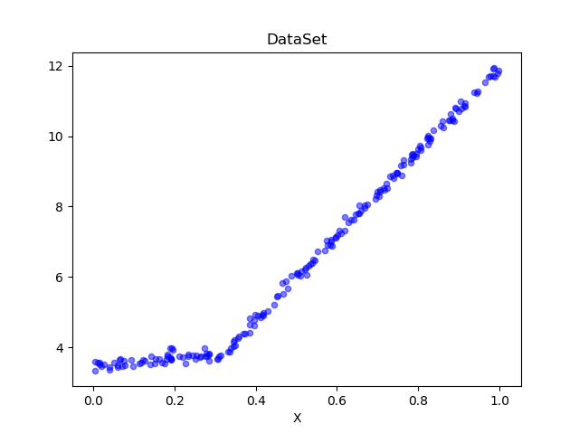
We can see that it is consistent with the image we introduced above. We use the model tree to process the code and generate the regression line.

Generate a model tree:

if __name__ == "__main__":
    # Model Tree
    myDat = loadDataSet('C:\\Users\\Administrator\\Desktop\\blog\\github\\AILearners\\data\\ml\\jqxxsz\\9.RegTrees\\exp2.txt')
    myMat = mat(myDat)
    myTree2 = createTree(myMat, modelLeaf, modelErr, ops=(1, 20))
    print(myTree2)

The results are as follows:

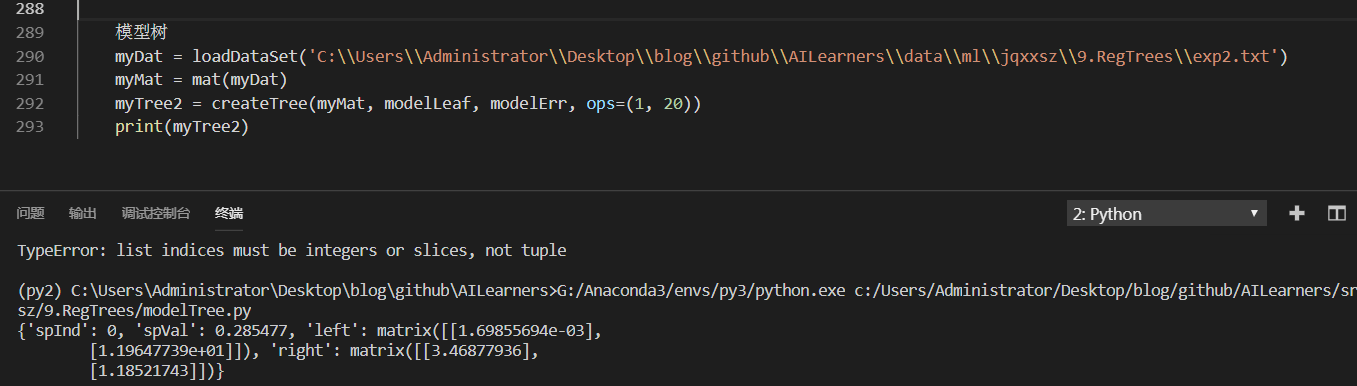
As you can see, the code creates two templates bounded by 0.285477. The original graph is actually divided into 0.3 segments with little error. The linear models generated by createTree() are y=3.468+1.1852x and y= 0.0016985+11.96477x, which are very close to the real models used to generate the data. The data are actually generated by the model y=3.5+1.0x and y=0+12x plus Gauss noise.

We can see the following figure:

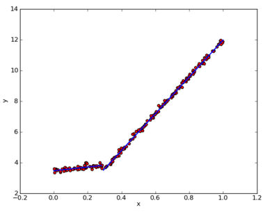
It can be seen that regression using model tree is good.

3. Case Study of Tree Regression Project

Project Case 1: Comparison of Tree Regression and Standard Regression

3.1. Project overview

The model tree, the regression tree and the general regression method are introduced before, and the following test is to find out which model is the best.

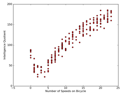
These models will be tested on a data set that deals with the relationship between human intelligence and bicycle speed. Of course, the data is false.

3.2. Development process

Collecting data: collecting data in any way
Prepare data: Numeric data is needed, nominal data should be mapped to binary data
Analytical data: Draw the results of two-dimensional visualization of the data, and generate the tree in a dictionary way.
Training Algorithms: Model Tree Construction
Test Algorithms: Use R^2 values on test data to analyze the effect of the model
Using algorithms: Using trained trees to make predictions, the predictions can also be used to do a lot of things.

Data storage format:

The data sets are bikeSpeedVsIq_test.txt and bikeSpeedVsIq_train.txt.
Data Set Download Address: Data Set Download

3.000000	46.852122
23.000000	178.676107
0.000000	86.154024
6.000000	68.707614
15.000000	139.737693

Analytical data: Draw the results of two-dimensional visualization of the data, and generate the tree in a dictionary way.

Training Algorithms: Model Tree Construction

Code for predicting with tree regression

# Regression Tree Test Case
# To be consistent with modelTreeEval(), keep two input parameters
def regTreeEval(model, inDat):
    """
    Desc:
        //Prediction of regression tree
    Args:
        model -- Specify the model, the optional value is the regression tree model or the model tree model, here is the regression tree.
        inDat -- Input test data
    Returns:
        float(model) -- Converting input model data to floating point returns
    """
    return float(model)


# Model Tree Test Case
# The input data is formatted and column 0 is added to the original data matrix. The values of the elements are all 1.
# That is to say, increasing the offset value is a routine with our previous simple linear regression, adding an offset.
def modelTreeEval(model, inDat):
    """
    Desc:
        //Prediction of Model Tree
    Args:
        model -- Input model, optional value is regression tree model or model tree model, here is model tree model.
        inDat -- Input test data
    Returns:
        float(X * model) -- The test data is multiplied by regression coefficient to get a predicted value, which is converted into floating point return.
    """
    n = shape(inDat)[1]
    X = mat(ones((1, n+1)))
    X[:, 1: n+1] = inDat
    # print X, model
    return float(X * model)


# Calculating the predicted results
# Given the tree structure, the function gives a predictive value for a single data point.
# modelEval refers to a function that predicts leaf nodes, specifying the type of tree to invoke the appropriate model on leaf nodes.
# This function traverses the whole tree from top to bottom until it hits the leaf node. Once it reaches the leaf node, it will be on the input data.
# Call the modelEval() function, which defaults to regTreeEval()
def treeForeCast(tree, inData, modelEval=regTreeEval):
    """
    Desc:
        //Predicting the tree of a particular model can be either a regression tree or a model tree.
    Args:
        tree -- Model of trained trees
        inData -- Input test data
        modelEval -- Predicted tree model type, optional value regTreeEval(Regression tree) or modelTreeEval(Model tree, default to regression tree
    Returns:
        //Return the predicted value
    """
    if not isTree(tree):
        return modelEval(tree, inData)
    if inData[tree['spInd']] <= tree['spVal']:
        if isTree(tree['left']):
            return treeForeCast(tree['left'], inData, modelEval)
        else:
            return modelEval(tree['left'], inData)
    else:
        if isTree(tree['right']):
            return treeForeCast(tree['right'], inData, modelEval)
        else:
            return modelEval(tree['right'], inData)


# Prediction results
def createForeCast(tree, testData, modelEval=regTreeEval):
    """
    Desc:
        //Call treeForeCast to predict the tree of a particular model, either a regression tree or a model tree.
    Args:
        tree -- Model of trained trees
        inData -- Input test data
        modelEval -- Predicted tree model type, optional value regTreeEval(Regression tree) or modelTreeEval(Model tree, default to regression tree
    Returns:
        //Return the predicted value matrix
    """
    m = len(testData)
    yHat = mat(zeros((m, 1)))
    # print yHat
    for i in range(m):
        yHat[i, 0] = treeForeCast(tree, mat(testData[i]), modelEval)
        # print "yHat==>", yHat[i, 0]
    return yHat

Test Algorithms: Use R^2 values on test data to analyze the effect of the model

The R ^ 2 judgment coefficient is the goodness of fit judgment coefficient, which reflects the proportion of the variation of independent variables in the variation of dependent variables in the regression model. For example, R^2=0.99999 indicates that 99.999% of the variation of dependent variable y is caused by variable x. When R^2=1, all observation points fall on the fitted line or curve; when R ^ 2 = 0, there is no linear or curve relationship between independent variable and dependent variable.

So we see that the closer R^2 is to 1.0, the better.

Using algorithms: Using trained trees to make predictions, the predictions can also be used to do a lot of things.

Specifically, we can refer to this complete code for writing: https://github.com/aimi-cn/AILearners/tree/master/src/py2.x/ml/jqxxsz/9.RegTrees/demo.py.

AIMI-CN AI Learning Exchange Group [1015286623] for more AI information
Sweep code plus group:

Share technology, enjoy life: our public number computer vision this trivial matter weekly push "AI" series of information articles, welcome your attention!