Read data and preprocess
import keras
from keras import layers
import numpy as np
from matplotlib import pyplot as plt
import pandas as pd
%matplotlib inline
Using TensorFlow backend.
# header=None means that the data file has no header, and the first line is the data.
data = pd.read_csv("./data/credit-a.csv", header=None)
data.head()
| 0 | 1 | 2 | 3 | 4 | 5 | 6 | 7 | 8 | 9 | 10 | 11 | 12 | 13 | 14 | 15 | |
|---|---|---|---|---|---|---|---|---|---|---|---|---|---|---|---|---|
| 0 | 0 | 30.83 | 0.000 | 0 | 0 | 9 | 0 | 1.25 | 0 | 0 | 1 | 1 | 0 | 202 | 0.0 | -1 |
| 1 | 1 | 58.67 | 4.460 | 0 | 0 | 8 | 1 | 3.04 | 0 | 0 | 6 | 1 | 0 | 43 | 560.0 | -1 |
| 2 | 1 | 24.50 | 0.500 | 0 | 0 | 8 | 1 | 1.50 | 0 | 1 | 0 | 1 | 0 | 280 | 824.0 | -1 |
| 3 | 0 | 27.83 | 1.540 | 0 | 0 | 9 | 0 | 3.75 | 0 | 0 | 5 | 0 | 0 | 100 | 3.0 | -1 |
| 4 | 0 | 20.17 | 5.625 | 0 | 0 | 9 | 0 | 1.71 | 0 | 1 | 0 | 1 | 2 | 120 | 0.0 | -1 |
# Viewing the Value of Characteristic Data
data.iloc[:, -1].unique()
array([-1, 1], dtype=int64)
# Shuffle data
# Generate an arbitrary unique index for this area
index = np.random.permutation(len(data))
# You can scramble it with the generated scrambled index
data = data.iloc[index ,:]
# Dividing data
x = data.iloc[:, 0:-1]
y = data.iloc[:, -1]
x.shape, y.shape
((653, 15), (653,))
Because the predicted value y is -1 to 1, and the output of Sigmoid + cross-entropy is between 01, so before training, y is processed and transformed to 01.
y = y.replace(-1, 0)
y.unique()
array([1, 0], dtype=int64)
# Previously, all I learned was to use DataFrame or Series directly.
type(x), type(y)
(pandas.core.frame.DataFrame, pandas.core.series.Series)
# It's also possible to use ndarray
x, y = x.values, y.values
type(x), type(y)
x.shape, y.shape
((653, 15), (653,))
# Converting y to data in 653 rows and 1 columns
y = y.reshape(-1, 1)
y.shape
(653, 1)
Establishment and training model
# It is also possible to replace input_dim with input_shape. The first dimension, None, indicates that any number of samples can be input.
model = keras.Sequential()
model.add(layers.Dense(128, input_shape=(15,), activation='relu'))
model.add(layers.Dense(128, activation='relu'))
model.add(layers.Dense(128, activation='relu'))
model.add(layers.Dense(1, activation='sigmoid'))
WARNING:tensorflow:From E:\MyProgram\Anaconda\envs\krs\lib\site-packages\tensorflow\python\framework\op_def_library.py:263: colocate_with (from tensorflow.python.framework.ops) is deprecated and will be removed in a future version.
Instructions for updating:
Colocations handled automatically by placer.
model.summary()
_________________________________________________________________
Layer (type)                 Output Shape              Param #
=================================================================
dense_1 (Dense)              (None, 128)               2048
_________________________________________________________________
dense_2 (Dense)              (None, 128)               16512
_________________________________________________________________
dense_3 (Dense)              (None, 128)               16512
_________________________________________________________________
dense_4 (Dense)              (None, 1)                 129
=================================================================
Total params: 35,201
Trainable params: 35,201
Non-trainable params: 0
_________________________________________________________________
model.compile(
    optimizer='adam',
    loss='binary_crossentropy',
    metrics=['acc']
)
history = model.fit(x, y, epochs=1000, verbose=0)
WARNING:tensorflow:From E:\MyProgram\Anaconda\envs\krs\lib\site-packages\tensorflow\python\ops\math_ops.py:3066: to_int32 (from tensorflow.python.ops.math_ops) is deprecated and will be removed in a future version.
Instructions for updating:
Use tf.cast instead.
Drawing training process
plt.plot(history.epoch, history.history.get('loss'), c='r')
plt.plot(history.epoch, history.history.get('acc'), c='b')
[<matplotlib.lines.Line2D at 0x144130b8>]
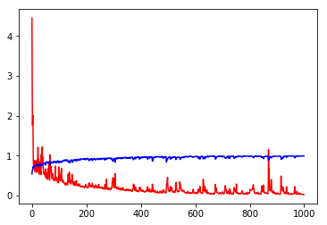
So many parameters, the results of Loss is really low, Acc is really high, but they are in the training set, can not objectively evaluate the model, the following is divided into training set and verification set to try.
Another attempt to segment data sets
k = int(len(x)*0.75)
x_train = x[:k]
x_test = x[k:]
y_train = y[:k]
y_test = y[k:]
x_train.shape, x_test.shape, y_train.shape, y_test.shape
((489, 15), (164, 15), (489, 1), (164, 1))
Be careful not to directly model.fit() here, or you will continue to train with the model you trained earlier, rebuild and recompile here, and then train again.
model = keras.Sequential()
model.add(layers.Dense(128, input_shape=(15,), activation='relu'))
model.add(layers.Dense(128, activation='relu'))
model.add(layers.Dense(128, activation='relu'))
model.add(layers.Dense(1, activation='sigmoid'))
model.compile(
    optimizer='adam',
    loss='binary_crossentropy',
    metrics=['acc']
)
history = model.fit(x_train, y_train, epochs=1000, verbose=0)
plt.plot(history.epoch, history.history.get('loss'), c='r')
plt.plot(history.epoch, history.history.get('acc'), c='b')
[<matplotlib.lines.Line2D at 0x144f61d0>]
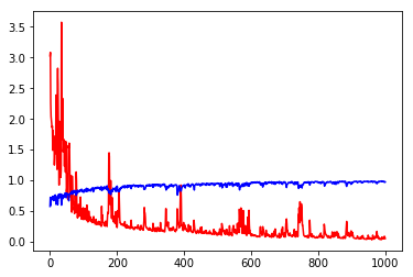
Using Keras model. evaluation () can easily get Performance evaluation on data sets. The results are Loss and accuracy.
# Performance on Training Sets
model.evaluate(x_train, y_train)
489/489 [==============================] - 0s 147us/step


[0.05114140091863878, 0.9754601228212774]
# Performance on Verification Sets
model.evaluate(x_test, y_test)
164/164 [==============================] - 0s 85us/step


[1.233076281663848, 0.8658536585365854]
You can see that over-fitting happened.
How to get Performance on verification set while training
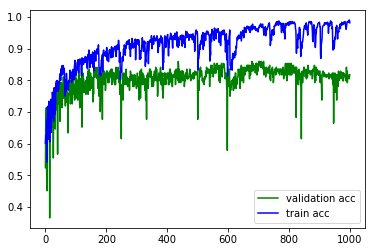
model = keras.Sequential()
model.add(layers.Dense(128, input_shape=(15,), activation='relu'))
model.add(layers.Dense(128, activation='relu'))
model.add(layers.Dense(128, activation='relu'))
model.add(layers.Dense(1, activation='sigmoid'))
model.compile(
    optimizer='adam',
    loss='binary_crossentropy',
    metrics=['acc']
)
# Adding validation_data here keeps Performance on the verification set for each epoch in the training process
history = model.fit(x_train, y_train, epochs=1000, validation_data=(x_test, y_test), verbose=0)
# Compare Acc (green) on the verification set with Acc (blue) on the training set.
plt.plot(history.epoch, history.history.get('val_acc'), c='g', label='validation acc')
plt.plot(history.epoch, history.history.get('acc'), c='b', label='train acc')
plt.legend() # Activation legend
<matplotlib.legend.Legend at 0x185f4eb8>