empirical orthogonal function analysis (EOF), also known as eigenvector analysis or principal component analysis, is a method to analyze the structural features in matrix data and extract the feature quantity of main data.

Import module

import cartopy.crs as ccrs
import cartopy.feature as cfeature
from netCDF4 import Dataset
import matplotlib.pyplot as plt
import numpy as np

from eofs.standard import Eof
from eofs.examples import example_data_path

import warnings
warnings.filterwarnings('ignore')

/home/lqy/anaconda3/lib/python3.8/site-packages/iris/config.py:139: UserWarning: Ignoring config item 'Resources':'test_data_dir' (section:option) as '/home/h05/itwl/projects/git/iris-test-data/test_data' is not a valid directory path.
  warnings.warn(msg.format(section, option, c_path))

North Atlantic geopotential height data in winter

North Atlantic oscillation (NAO) was discovered by Sir Gilbert Walker (G. Walker) in 1920. One of the three major oscillations refers to the reverse change relationship of air pressure between Azores high pressure and Icelandic low pressure, that is, when the air pressure in Azores is high, the air pressure in Iceland is low, and vice versa. NAO is the most significant atmospheric mode in the North Atlantic region. The most prominent climate impact is mainly in North America and Europe, but it may also have a certain impact on the climate of other regions such as Asia.

# Read geopotential height data using the netCDF4 module. The file contains
# December-February averages of geopotential height at 500 hPa for the
# European/Atlantic domain (80W-40E, 20-90N).
filename = '../input/eof7091/hgt_djf.nc'
ncin = Dataset(filename, 'r')
z_djf = ncin.variables['z'][:]
lons = ncin.variables['longitude'][:]
lats = ncin.variables['latitude'][:]
ncin.close()

# Compute anomalies by removing the time-mean.
z_djf_mean = z_djf.mean(axis=0)
z_djf = z_djf - z_djf_mean

# Create an EOF solver to do the EOF analysis. Square-root of cosine of
# latitude weights are applied before the computation of EOFs.
coslat = np.cos(np.deg2rad(lats)).clip(0., 1.)
wgts = np.sqrt(coslat)[..., np.newaxis]
solver = Eof(z_djf, weights=wgts)

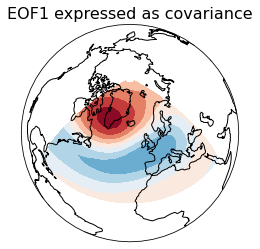
# Retrieve the leading EOF, expressed as the covariance between the leading PC
# time series and the input SLP anomalies at each grid point.
eof1 = solver.eofsAsCovariance(neofs=1)

# Plot the leading EOF expressed as covariance in the European/Atlantic domain.
clevs = np.linspace(-75, 75, 11)
proj = ccrs.Orthographic(central_longitude=-20, central_latitude=60)
ax = plt.axes(projection=proj)
ax.set_global()
ax.coastlines()
ax.contourf(lons, lats, eof1.squeeze(), levels=clevs,
            cmap=plt.cm.RdBu_r, transform=ccrs.PlateCarree())
plt.title('EOF1 expressed as covariance', fontsize=16)

plt.show()

There is a significant negative correlation between the pressure changes of the two atmospheric activity centers in the North Atlantic (Iceland low and Azores high); When the Icelandic low pressure deepens, the Azores high pressure strengthens, or when the Icelandic low pressure is filled, the Azores high pressure weakens. G. Walker called this phenomenon the North Atlantic oscillation (NAO). The strong North Atlantic Oscillation indicates that the pressure difference between the two active centers is large, and the westerly wind in the middle latitude of the North Atlantic is strong, which is a high exponential circulation. At this time, both the Gulf of Mexico warm current and the Labrador cold current increased, and northwest Europe and the southeastern United States were affected by the strong warm ocean current, resulting in a warm winter; At the same time, the east coast of Canada and the West Bank of Greenland, which are controlled by the cold current, are very cold. On the contrary, the North Atlantic oscillation is weak, indicating that the pressure difference between the two active centers is small, and the North Atlantic upwesterly wind is weakened, which is a low exponential circulation. At this time, there will be cold winter in northwest Europe and the southeast of the United States, while the east coast of Canada and the West Bank of Greenland are relatively warm.

Pacific SST anomaly data

El Ni ñ o phenomenon refers to the abnormal warming of the sea water in the eastern Pacific every few years. It is the warming stage of the eastern Pacific in the El Ni ñ o-Southern Oscillation (ENSO). It is related to the warm ocean currents generated at the equator of the central Pacific and the eastern Pacific (about 120 degrees west longitude and the international day exchange line). El Nino Southern Oscillation refers to the high and low temperature cycle of sea surface temperature at the equator of the central and eastern Pacific. El Nino phenomenon is caused by high pressure in the Western Pacific and low pressure in the eastern Pacific. The low temperature phase of El Nino Southern oscillation is called La Nina phenomenon (also known as anti El Nino phenomenon), which is caused by the higher than average sea surface temperature in the eastern Pacific, the lower pressure in the Western Pacific and the higher pressure in the eastern Pacific.

"""
Compute and plot the leading EOF of sea surface temperature in the
central and northern Pacific during winter time.

The spatial pattern of this EOF is the canonical El Nino pattern, and
the associated time series shows large peaks and troughs for well-known
El Nino and La Nina events.
"""
filename = '../input/eof7091/sst_ndjfm_anom.nc'
ncin = Dataset(filename, 'r')
sst = ncin.variables['sst'][:]
lons = ncin.variables['longitude'][:]
lats = ncin.variables['latitude'][:]
ncin.close()

# Create an EOF solver to do the EOF analysis. Square-root of cosine of
# latitude weights are applied before the computation of EOFs.
coslat = np.cos(np.deg2rad(lats))
wgts = np.sqrt(coslat)[..., np.newaxis]
solver = Eof(sst, weights=wgts)

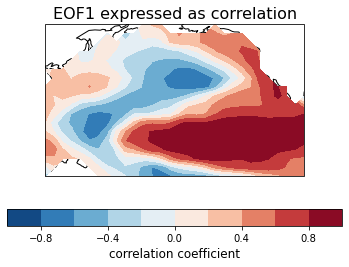
# Retrieve the leading EOF, expressed as the correlation between the leading
# PC time series and the input SST anomalies at each grid point, and the
# leading PC time series itself.
eof1 = solver.eofsAsCorrelation(neofs=1)
pc1 = solver.pcs(npcs=1, pcscaling=1)

# Plot the leading EOF expressed as correlation in the Pacific domain.
clevs = np.linspace(-1, 1, 11)
ax = plt.axes(projection=ccrs.PlateCarree(central_longitude=190))
fill = ax.contourf(lons, lats, eof1.squeeze(), clevs,
                   transform=ccrs.PlateCarree(), cmap=plt.cm.RdBu_r)
ax.add_feature(cfeature.LAND, facecolor='w', edgecolor='k')
cb = plt.colorbar(fill, orientation='horizontal')
cb.set_label('correlation coefficient', fontsize=12)
plt.title('EOF1 expressed as correlation', fontsize=16)

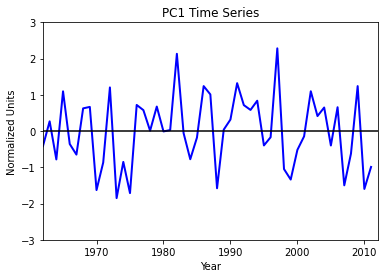
# Plot the leading PC time series.
plt.figure()
years = range(1962, 2012)
plt.plot(years, pc1, color='b', linewidth=2)
plt.axhline(0, color='k')
plt.title('PC1 Time Series')
plt.xlabel('Year')
plt.ylabel('Normalized Units')
plt.xlim(1962, 2012)
plt.ylim(-3, 3)
plt.show()